Ranking Models Across a Benchmark: From Mean to IQM

You have run a set of models across a benchmark and need a single aggregate ranking. Averaging the raw scores is the obvious first step, but it has two failure modes: metrics on different scales assign weight by numeric range rather than model quality, and lower-is-better metrics like RMSE reward higher values when averaged raw. This tutorial covers normalization and three aggregation methods — mean, trimmed mean, and IQM — that illustrate a set of tools to have some first insights into cross-dataset performance of models.

Note

This tutorial covers normalization, mean aggregation, trimmed mean aggregation, and bootstrap confidence intervals from multiple seeds. For pairwise probability statements (“what is the chance Model-B genuinely outperforms Model-A on a future task?”) see the Bayesian comparison tutorial. For win-rate and consistency shape across datasets see the performance profiles tutorial.

import warnings
warnings.filterwarnings("ignore")

import numpy as np
import pandas as pd
import matplotlib.pyplot as plt
import evaluma

1. Why normalization comes first

Aggregate scores only make sense when all scores live on a common scale and point in the same direction. When one dataset reports accuracy in [0, 1] and another reports RMSE that can reach 100, an unweighted mean is dominated by the RMSE dataset simply because its numeric range is larger. Direction compounds the problem: a raw mean treats higher as always better, so a model with high RMSE gets rewarded for what is actually poor performance.

The 3×3 toy example

To illustrate this, we will look at a small toy example with three models and three datasets.

df_toy = pd.DataFrame({
    "model":   ["Model-1"] * 3 + ["Model-2"] * 3 + ["Model-3"] * 3,
    "dataset": ["Dataset-A", "Dataset-B", "Dataset-C"] * 3,
    "metric":  ["accuracy", "f1", "rmse"] * 3,
    "score":   [0.72, 0.65, 12.0,
                0.84, 0.58, 45.0,
                0.61, 0.79, 28.0],
})
df_toy.pivot(index="model", columns="dataset", values="score")

dataset	Dataset-A	Dataset-B	Dataset-C
model
Model-1	0.72	0.65	12.0
Model-2	0.84	0.58	45.0
Model-3	0.61	0.79	28.0

Dataset-A: classification accuracy (0–1, higher is better). Dataset-B: F1 score (0–1, higher is better). Dataset-C: RMSE (0–∞, lower is better).

Average the three columns without any preprocessing:

raw_means = (
    df_toy.groupby("model")["score"]
    .mean()
    .sort_values(ascending=False)
    .rename("raw mean")
    .reset_index()
)
raw_means

	model	raw mean
0	Model-2	15.473333
1	Model-3	9.800000
2	Model-1	4.456667

Model-2 ranks first because its RMSE of 45 dwarfs the accuracy and F1 scores in [0, 1], giving it outsized weight in the raw mean regardless of model quality. The direction problem layers on top: because higher is treated as better, that RMSE of 45 counts as a large positive contribution even though it represents the worst performance on Dataset-C. Normalization resolves both issues by mapping each dataset to a common [0, 1] scale and flipping lower-is-better metrics so that higher always means better.

Loading with evaluma

evaluma.load_df() handles both steps: passing metric_direction={"Dataset-C": "min"} negates RMSE before normalization so that lower RMSE maps to a higher normalized value, and norm_ref_low / norm_ref_high set the scale endpoints per dataset.

bench_toy = evaluma.load_df(
    df_toy,
    model="model", dataset="dataset", metric="metric", score="score",
    norm_ref_low={"Dataset-A": 0.0, "Dataset-B": 0.0, "Dataset-C": 0.0},
    norm_ref_high={"Dataset-A": 1.0, "Dataset-B": 1.0, "Dataset-C": 100.0},
    metric_direction={"Dataset-C": "min"},
)
bench_toy.scores_.round(3)

	Dataset-A	Dataset-B	Dataset-C
model
Model-1	0.72	0.65	0.88
Model-2	0.84	0.58	0.55
Model-3	0.61	0.79	0.72

With norm_ref_high={"Dataset-C": 100.0}, a perfect RMSE of 0 maps to 1.0 and an RMSE of 100 maps to 0.0. Model-1’s RMSE of 12 becomes \((100 - 12) / 100 = 0.88\).

The normalized mean now makes sense:

norm_means = bench_toy.aggregate_ranking(agg="mean").table.rename(
    columns={"score": "normalized mean"}
)
norm_means["normalized mean"] = norm_means["normalized mean"].round(3)
norm_means

	model	normalized mean
0	Model-1	0.750
1	Model-3	0.707
2	Model-2	0.657

Model-1 now ranks first, despite middling accuracy (0.72) and F1 (0.65). Its strong RMSE translates to a normalized score of 0.88, giving it the highest mean of 0.750. The ordering now reflects model quality rather than metric scale and direction.

Warning

Passing norm_ref_low=0.0, norm_ref_high=1.0 as scalars is only valid when all raw scores already lie in [0, 1]. For RMSE or other unbounded metrics, always provide per-dataset bounds via a dict, or use metric_type_bounds. evaluma emits a UserWarning when bounds are not provided explicitly.

2. Mean aggregation: the baseline

For a benchmark where all datasets use the same metric and all scores already lie in a common range, mean aggregation is a natural starting point. The 5-model × 8-dataset synthetic benchmark below uses accuracy throughout (higher is better, scores in [0.13, 0.97]).

Two models have a bimodal score distribution: Model-A is strong on three datasets (D01–D03 ≈ 0.95) and weak on the remaining five (D04–D08 ≈ 0.42), while Model-B is the mirror image, weak on D01–D03 (≈ 0.15) and strong on D04–D08 (≈ 0.82). Models C, D, and E are stable across all datasets.

rng = np.random.RandomState(42)
datasets = [f"D{i:02d}" for i in range(1, 9)]

scores_dict = {
    "Model-A": np.concatenate([rng.uniform(0.93, 0.97, 3), rng.uniform(0.40, 0.44, 5)]),
    "Model-B": np.concatenate([rng.uniform(0.13, 0.17, 3), rng.uniform(0.80, 0.84, 5)]),
    "Model-C": rng.uniform(0.70, 0.74, 8),
    "Model-D": rng.uniform(0.58, 0.62, 8),
}
scores_dict["Model-E"] = np.clip(
    scores_dict["Model-D"] + rng.normal(0, 0.01, 8), 0.0, 1.0
)

rows = [
    {"model": m, "dataset": d, "metric": "acc", "score": float(s)}
    for m, sc in scores_dict.items()
    for d, s in zip(datasets, sc)
]
df_bench = pd.DataFrame(rows)

bench = evaluma.load_df(
    df_bench,
    model="model", dataset="dataset", metric="metric", score="score",
    norm_ref_low=0.0, norm_ref_high=1.0,
)

With scores already in [0, 1] and explicit scalar bounds, normalization is the identity. The score matrix:

bench.scores_.round(3)

	D01	D02	D03	D04	D05	D06	D07	D08
model
Model-A	0.945	0.968	0.959	0.424	0.406	0.406	0.402	0.435
Model-B	0.154	0.158	0.131	0.839	0.833	0.808	0.807	0.807
Model-C	0.712	0.721	0.717	0.712	0.724	0.706	0.712	0.715
Model-D	0.598	0.611	0.588	0.601	0.604	0.582	0.604	0.587
Model-E	0.592	0.608	0.582	0.619	0.604	0.571	0.613	0.575

Mean ranking computed directly from the normalized matrix:

palette = {
    "Model-A": "#2563EB", "Model-B": "#16A34A",
    "Model-C": "#D97706", "Model-D": "#DC2626", "Model-E": "#7C3AED",
}

mean_ranking = bench.aggregate_ranking(agg="mean").table.rename(columns={"score": "mean"})
mean_ranking.insert(0, "rank", range(1, len(mean_ranking) + 1))
mean_ranking["mean"] = mean_ranking["mean"].round(3)
mean_ranking

	rank	model	mean
0	1	Model-C	0.715
1	2	Model-A	0.618
2	3	Model-D	0.597
3	4	Model-E	0.595
4	5	Model-B	0.567

The normalized mean ranking places Model-C first. However, the aggregate ranking can hide important information that only a more careful per-dataset look reveals.

3. When mean misleads

Plotting each model’s score on every dataset makes a pattern visible that the aggregate table hides.

model_order = ["Model-A", "Model-B", "Model-C", "Model-D", "Model-E"]
fig, ax = plt.subplots(figsize=(10, 4))
x = np.arange(len(datasets))
width = 0.14
offsets = np.linspace(-2, 2, 5) * width

for i, model in enumerate(model_order):
    vals = bench.scores_.loc[model].values
    ax.bar(x + offsets[i], vals, width, label=model, color=palette[model])

ax.set_xticks(x)
ax.set_xticklabels(datasets, fontsize=9)
ax.set_ylim(0, 1.1)
ax.set_xlabel("Dataset")
ax.set_ylabel("Normalized score")
ax.set_title(
    "Model-A peaks on D01–D03 then falls below all others; "
    "Model-B dips on D01–D03 then leads on D04–D08"
)
ax.legend(ncol=5, fontsize=9)
plt.tight_layout()
plt.show()

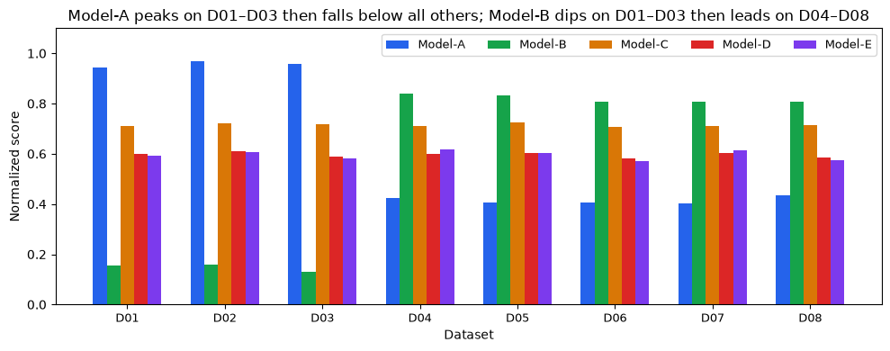
From the bar plot we can see that Model-A (blue) dominates the other models on datasets D01–D03 on the left. However, on the remaining five datasets it performs strictly worse than all other models. Its overall strong mean ranking is almost entirely a product of those first three datasets.

Model-B (green) shows the mirror image. It dips to 0.13–0.17 on D01–D03, then scores well above Model-A on D04–D08, where five of the eight datasets live. Its mean is suppressed by the same three datasets that inflate Model-A’s.

Mean aggregation treats all eight datasets as equally informative about a model’s typical performance. Three outlier datasets move the aggregate ranking in ways that might obscure how a model performs on representative tasks.

Note

This failure mode arises whenever any model has a bimodal score distribution across the benchmark, where it performs strong on a few tasks and considerably weaker on the others. Mean aggregation cannot tell the difference between a model that’s consistently mediocre and one that’s strong on most tasks but has a few outlier failures. The two patterns can produce identical mean scores while pointing to very different models.

4. Trimmed mean aggregation: a robust point estimate

If experiment results are dominated by some outliers, it can be more meaningful to look at a different mode of aggregation. The 25% trimmed mean is a more robust statistic than the mean: it sorts each model’s scores across datasets from lowest to highest, discards the bottom quarter and the top quarter, then averages what remains — the middle 50%.

The concept of trimming 25% from each extreme for benchmark aggregation was introduced for RL benchmarking in Agarwal et al. (2021, NeurIPS). aggregate_ranking(agg="trimmed_mean") applies this as a dataset-level summary statistic: one score per dataset (or the mean over seeds if multiple runs are present). See section 5 for the Agarwal IQM on the full run×dataset array with bootstrap CIs.

With 8 datasets, the trim removes 2 datasets at each extreme, leaving the middle 4 to be averaged.

For Model-A, two of its three highest-scoring datasets land in the top 2 that get trimmed — but crucially, one high-scoring dataset (D03 ≈ 0.945) survives into the middle 4, because there are three outlier datasets but only two trimming slots at each end. Similarly for Model-B, one low-scoring dataset (D03 ≈ 0.158) survives in the middle 4. This realistic partial-trim is worth noticing: the trimmed mean moderates the extremes without requiring them to vanish entirely.

Formal definition

For a model’s normalized scores across datasets sorted as \(x_{(1)} \le x_{(2)} \le \cdots \le x_{(n)}\):

\[\text{trimmed mean} = \frac{1}{n/2} \sum_{i=\lfloor n/4 \rfloor + 1}^{\lceil 3n/4 \rceil} x_{(i)}\]

For \(n = 8\): average positions 3 through 6 (four datasets). Implemented as scipy.stats.trim_mean(row, proportiontocut=0.25).

trimmed_result = bench.aggregate_ranking(agg="trimmed_mean")
median_result = bench.aggregate_ranking(agg="median")
trimmed_result.table.round(3)

	model	score
0	Model-C	0.714
1	Model-B	0.645
2	Model-D	0.598
3	Model-E	0.597
4	Model-A	0.552

Note

aggregate_ranking() returns a point estimate only — a descriptive summary of benchmark performance on the observed datasets. No confidence interval is provided, because with one run per dataset there is no seed variance to estimate. If you have multiple runs per dataset and want to assess whether the ranking is robust to seed choice, see section 5.

Placing mean, trimmed mean, and median side by side reveals the ranking shift:

mean_rank_df = bench.aggregate_ranking(agg="mean").table.rename(columns={"score": "mean"})
mean_rank_df.insert(0, "mean_rank", range(1, len(mean_rank_df) + 1))
mean_rank_df["mean"] = mean_rank_df["mean"].round(3)

trimmed_rank_df = trimmed_result.table[["model", "score"]].rename(
    columns={"score": "trimmed_mean"}
).copy()
trimmed_rank_df.insert(0, "trimmed_rank", range(1, len(trimmed_rank_df) + 1))
trimmed_rank_df["trimmed_mean"] = trimmed_rank_df["trimmed_mean"].round(3)

median_rank_df = median_result.table[["model", "score"]].rename(
    columns={"score": "median"}
).copy()
median_rank_df.insert(0, "median_rank", range(1, len(median_rank_df) + 1))
median_rank_df["median"] = median_rank_df["median"].round(3)

comparison = (
    mean_rank_df
    .merge(trimmed_rank_df, on="model")
    .merge(median_rank_df, on="model")
)
comparison.sort_values("trimmed_rank").reset_index(drop=True)

	mean_rank	model	mean	trimmed_rank	trimmed_mean	median_rank	median
0	1	Model-C	0.715	1	0.714	2	0.713
1	5	Model-B	0.567	2	0.645	1	0.807
2	3	Model-D	0.597	3	0.598	3	0.599
3	4	Model-E	0.595	4	0.597	4	0.598
4	2	Model-A	0.618	5	0.552	5	0.429

Model-A drops from second by mean to last by trimmed mean. After trimming, two of its three high-scoring outlier datasets (≈ 0.95–0.97) are removed along with two of its low-scoring stable datasets (≈ 0.40), leaving a middle four that averages to about 0.55. By median the score falls further to ≈ 0.43, reflecting its typical performance on the five representative datasets.

Model-B moves in the opposite direction. Its three low-scoring outlier datasets (≈ 0.13–0.17) suppress the mean, but after trimming only one survives in the middle four alongside three strong datasets (≈ 0.81). Median bypasses the low outliers entirely and returns ≈ 0.81, moving Model-B to first place.

Model-C is stable throughout, ranking first by mean and trimmed mean and second by median with almost no change in score. Models D and E shift at most one position; their uniform scores mean no aggregation method can separate them by much.

The median is not a strict improvement over trimmed mean — by discarding 50% of data it throws away half the benchmark’s representative tasks entirely. Trimmed mean is a principled middle ground: aggressive enough to neutralize true outliers while retaining more of the benchmark’s evidence. The consistent direction of the B vs A reversal across both methods is itself informative: it signals that the reversal is genuine and not an artefact of a particular trimming threshold.

Aggregate rankings summarize performance across the whole benchmark and can obscure large differences in how models perform on individual tasks. A model that ranks well overall may underperform on the tasks that matter most for a specific application, so it is worth checking per-dataset scores alongside the aggregate before making a deployment decision.

5. Statistical inference with multiple seeds

A trimmed mean point estimate answers one question: given these exact 8 datasets and these exact experiment runs, how do the models rank? It says nothing about whether the ranking would hold if there were multiple random seeded runs per model on each dataset, which turns into a question about seed-variance reliability, not benchmark composition.

Why shift from trimmed mean to IQM? Agarwal et al. (2021) wrote rliable in response to a specific problem in deep reinforcement learning: a single training run of the same algorithm can produce very different performance depending on the random seed used to initialize the network and the environment. Reporting the result from one seed was common practice, but it left rankings unstable — run the experiment again with a different seed and the ranking could change. Agarwal et al. proposed IQM combined with stratified bootstrap confidence intervals as a principled standard for multi-seed RL evaluation. For a more detailed explanation see their paper, or this illustrative blog post by one of the authors.

Section 4’s trimmed mean and IQM both apply a 25% trim, but to different inputs:

• Section 4 computes one point estimate per dataset (either the raw score or the mean over seeds if multiple runs exist), then trims outlier datasets — the most extreme point estimates in the benchmark.

• Section 5 concatenates all seed × dataset scores into a single flat array per model, then trims the outer 25% of outlier runs — individual seed × dataset pairs that deviate most from the model’s typical performance.

When seed variance is small, the two procedures return similar point estimates. Their key difference is what they measure: the trimmed mean describes aggregate performance on this benchmark; IQM + bootstrap CIs answer whether that aggregate is reproducible across different random seeds.

To assess seed reliability, you need multiple runs per dataset. With three seeds per (model, dataset) pair, iqm_ranking() implements the Agarwal et al. (2021) IQM on the full run × dataset flat array: all seeds × datasets normalized scores per model are concatenated into a single vector, the outer 25% are trimmed, and the remainder is averaged. A stratified bootstrap constructs 95% CIs by resampling seeds independently within each dataset stratum (following the rliable methodology of Agarwal et al. 2021) and recomputing IQM on each resample.

With 3 seeds and 8 datasets the flat array has \(3 \times 8 = 24\) values per model. Trimming 25% removes 6 from each end, leaving the middle 12 to average. The stratified bootstrap draws 3 seed scores with replacement per dataset separately, preserving the dataset structure while capturing seed variance.

The CI width reflects how sensitive the IQM is to which seeds happened to be run. A narrow CI means the ranking is robust to seed choice; a wide CI means different seeds could plausibly reorder the models.

Constructing a multi-seed benchmark

We extend the same 5-model × 8-dataset benchmark from sections 2–4 by adding three seeds per (model, dataset) cell. To produce visually distinct CI widths, we use model-specific seed variance: Model-B’s outlier datasets (D01–D03) have high variance (σ = 0.11) to simulate a model whose performance is sensitive to initialization on those tasks; Model-C is stable everywhere (σ = 0.01); the others have moderate variance (σ = 0.02–0.04).

outlier_datasets = {"D01", "D02", "D03"}
model_sigma = {
    "Model-A": {"outlier": 0.04, "stable": 0.02},
    "Model-B": {"outlier": 0.11, "stable": 0.02},
    "Model-C": {"outlier": 0.01, "stable": 0.01},
    "Model-D": {"outlier": 0.02, "stable": 0.02},
    "Model-E": {"outlier": 0.02, "stable": 0.02},
}

rng2 = np.random.RandomState(99)
rows_seeded = []
for m, sc in scores_dict.items():
    sigs = model_sigma[m]
    for d, base in zip(datasets, sc):
        sigma = sigs["outlier"] if d in outlier_datasets else sigs["stable"]
        for seed_id in [1, 2, 3]:
            score = float(np.clip(base + rng2.normal(0, sigma), 0.0, 1.0))
            rows_seeded.append(
                {"model": m, "dataset": d, "metric": "acc", "score": score, "seed": seed_id}
            )
df_seeded = pd.DataFrame(rows_seeded)

bench_runs = evaluma.load_df(
    df_seeded,
    model="model", dataset="dataset", metric="metric", score="score",
    seed="seed",
    norm_ref_low=0.0, norm_ref_high=1.0,
)

Passing seed="seed" tells evaluma to retain all per-seed rows as raw runs rather than averaging them. bench_runs.scores_ still exposes a (5, 8) mean-aggregated matrix for inspection; iqm_ranking() operates on the full run-level data.

IQM with stratified bootstrap CIs

iqm_runs = bench_runs.iqm_ranking(random_state=42)
iqm_runs.table.round(3)

	model	IQM	CI_low	CI_high
0	Model-C	0.715	0.712	0.719
1	Model-B	0.666	0.638	0.691
2	Model-E	0.604	0.595	0.612
3	Model-D	0.599	0.591	0.604
4	Model-A	0.555	0.549	0.561

The point estimates closely match the trimmed mean values from section 4. The two quantities differ conceptually — the flat-array IQM trims from 24 values while the dataset-level trimmed mean trims from 8 mean scores — but agree closely when seed variance is small.

# Compare aggregate_ranking point estimate with IQM point estimate
agg_pts = bench_runs.aggregate_ranking(agg="trimmed_mean").table.rename(
    columns={"score": "trimmed_mean"}
)
iqm_pts = iqm_runs.table[["model", "IQM"]].copy()
pd.merge(agg_pts, iqm_pts, on="model").round(3)

	model	trimmed_mean	IQM
0	Model-C	0.714	0.715
1	Model-B	0.652	0.666
2	Model-E	0.605	0.604
3	Model-D	0.597	0.599
4	Model-A	0.554	0.555

The CI plot makes the uncertainty explicit:

fig = iqm_runs.plot(
    figsize=(6, 3.5),
    model_colors=[palette[m] for m in iqm_runs.table["model"].tolist()],
    title="IQM scores with 95% stratified-bootstrap CIs (3 seeds × 8 datasets)",
)
plt.tight_layout()
plt.show()

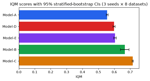
The CI widths directly reflect the model-specific seed variance we specified:

• Model-B has the widest CI by far. Its D01–D03 scores vary substantially across seeds (σ = 0.11): bootstrap resamples that happen to draw more of the weak seed runs on those datasets push B’s IQM down, while resamples that avoid them push it up. B is genuinely strong on D04–D08, but its aggregate IQM is sensitive to which seeds happened to run on the outlier datasets.

• Model-C has the narrowest CI. Stable scores across all datasets and all seeds (σ = 0.01) mean that bootstrap resampling changes almost nothing.

• Models D and E have overlapping CIs and nearly identical point estimates. Their scores differ by less than 0.02 per dataset, so the bootstrap cannot separate them — claiming a definitive ordering between them would be overconfident.

• Model-A has a narrow CI. Its outlier datasets (D01–D03) are near ceiling (σ = 0.04 on ≈ 0.95), so the absolute range of resampled scores is compressed; the stable datasets (σ = 0.02) contribute little variance.

Model-B’s wide CI is not uncertainty about measurement noise — it is uncertainty about which seeds happened to run. Different initializations on D01–D03 could plausibly shift B’s IQM by as much as ±0.03.

Note

Overlapping CIs do not mean the models are equivalent — only that the ranking is not well-supported given these particular seed runs. When the ordering matters for a deployment decision, use bench.bayesian_comparison() to get a direct probability that one model outperforms the other on a new task. See the Bayesian tutorial for a worked example.

6. Applying to GeoBenchV2

GeoBenchV2 (Simumba et al., 2026) evaluates 14 pretrained backbone models on 19 geospatial datasets spanning land cover classification, crop detection, object detection, and scene understanding — a deliberately diverse benchmark with no single dominant task type. One dataset (biomassters) reports RMSE (lower is better); all others report F1, Jaccard index, accuracy, or mean average precision (higher is better). Each backbone was evaluated with multiple random seeds.

The paper’s headline finding is that no single model dominates: EO-specialized backbones (TerraMind, Prithvi, Clay) trained on multi-spectral satellite imagery lead on multi-spectral classification tasks, while natural-image backbones (ConvNeXt, DINOv3) trained on large RGB datasets lead on high-resolution and scene-level tasks. This per-task picture is one takeaway — but the IQM aggregate tells a different story about which backbones generalize best across the whole benchmark.

Our normalization uses fixed [0, 1] bounds per dataset. The paper uses reference-anchored normalization (scoring each backbone relative to a reference model), so absolute IQM values here will differ from the paper’s leaderboard numbers; relative rankings are directly comparable.

df_raw = pd.read_csv("../../results_and_parameters.csv")

full_coverage = (
    df_raw.groupby("backbone")["dataset"]
    .nunique()
    .pipe(lambda s: s[s == 19].index)
    .tolist()
)
df_geo = df_raw[df_raw["backbone"].isin(full_coverage)].copy()

bench_geo = evaluma.load_df(
    df_geo,
    model="backbone",
    dataset="dataset",
    metric="Metric",
    score="test metric",
    seed="Seed",
    norm_ref_low=0.0,
    norm_ref_high=1.0,
    metric_direction={"biomassters": "min"},
)

seed="Seed" retains all per-seed rows as raw runs. bench_geo.scores_ exposes a mean-aggregated matrix for reference, but iqm_ranking() operates on the full run-level data to compute the flat-array IQM and stratified bootstrap CIs.

metric_direction={"biomassters": "min"} negates RMSE before normalization so a lower RMSE maps to a higher normalized score — consistent with all other datasets.

Mean vs IQM ranking

iqm_geo = bench_geo.iqm_ranking(random_state=42)

mean_geo = bench_geo.aggregate_ranking(agg="mean").table.rename(columns={"score": "mean"})
mean_geo.insert(0, "mean_rank", range(1, len(mean_geo) + 1))
mean_geo["mean"] = mean_geo["mean"].round(3)

iqm_geo_df = iqm_geo.table[["model", "IQM"]].copy()
iqm_geo_df.insert(0, "iqm_rank", range(1, len(iqm_geo_df) + 1))
iqm_geo_df["IQM"] = iqm_geo_df["IQM"].round(3)

comparison_geo = mean_geo.merge(iqm_geo_df, on="model")
comparison_geo["rank_diff"] = comparison_geo["mean_rank"] - comparison_geo["iqm_rank"]
comparison_geo.sort_values("iqm_rank").reset_index(drop=True)

	mean_rank	model	mean	iqm_rank	IQM	rank_diff
0	1	convnext_xlarge_fb_in22k	0.514	1	0.544	0
1	2	convnext_large_fb_in22k	0.507	2	0.543	0
2	6	dinov3_convnext_large	0.503	3	0.542	3
3	7	dinov3_vitl16	0.496	4	0.538	3
4	3	clay_v1_base	0.506	5	0.533	-2
5	5	terramind_v1_large	0.503	6	0.531	-1
6	4	satlas_swin_b_sentinel2_si_ms	0.504	7	0.530	-3
7	8	dofa_large_patch16_224	0.495	8	0.527	0
8	9	prithvi_eo_v2_600_tl	0.493	9	0.518	0
9	12	satlas_swin_b_naip_si_rgb	0.485	10	0.518	2
10	11	terramind_v1_base	0.486	11	0.511	0
11	10	prithvi_eo_v2_300_tl	0.489	12	0.508	-2
12	13	ssl4eos12_resnet50_sentinel2_all_decur	0.466	13	0.477	0
13	14	resnet50	0.456	14	0.473	0

The two most striking rank shifts mirror the toy example from sections 2–4:

DINOv3 models rise +3 positions each (dinov3_convnext_large: rank 6 → 3; dinov3_vitl16: rank 7 → 4). Their mean scores are suppressed by a handful of geospatial tasks where EO-specialized backbones dominate — multi-spectral classification tasks that suit Sentinel-2 pretrained models. After IQM trims those outlier-low datasets, DINOv3’s genuine broad performance across the benchmark is revealed as stronger than the mean implied. This is the Model-B pattern: a few outlier tasks suppress the mean.

satlas_swin_b_sentinel2_si_ms drops 3 positions (rank 4 → 7). Its Sentinel-2 pretraining boosts performance on specific multi-spectral tasks — exactly the datasets where DINOv3 is weak. Those outlier-high datasets inflate its mean; after IQM trims them, its typical performance across the benchmark is lower than the mean suggested. This is the Model-A pattern: a few specialized datasets inflate the mean.

clay_v1_base also drops 2 positions for the same reason. The remaining backbones are stable across both aggregations.

The top two positions are occupied by convnext_xlarge and convnext_large under both methods — these natural-image backbones generalize broadly enough that no small set of outlier tasks dominates their aggregate.

IQM with confidence intervals

fig = iqm_geo.plot(
    figsize=(9, 5),
    title="GeoBench — IQM ranking with 95% stratified-bootstrap CIs (19 datasets)",
)
plt.tight_layout()
plt.show()

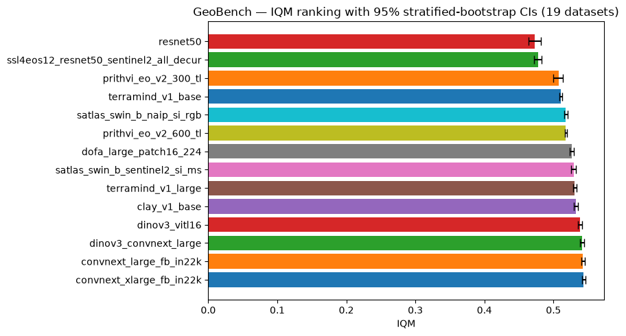
Most backbones have narrow CIs, meaning the IQM ranking is stable across seeds for GeoBench: the top-4 and bottom-2 positions would be hard to change with different random initializations. The widest CIs belong to resnet50 and prithvi_eo_v2_300_tl, which show more variance across seeds — possibly because smaller or less-pretrained models are more sensitive to initialization on geospatial tasks. For a direct probability statement — “how likely is backbone X to outperform backbone Y on a new geospatial task?” — use bench_geo.bayesian_comparison() as shown in the Bayesian tutorial. For win-rate and consistency profiles see the performance profiles tutorial.

---

Summary

In this tutorial we have looked at the arguably most common method of aggregating model performance scores across a set of datasets to get higher level summary statistics and information about broad model performance. A few takeaways are:

• Normalize before aggregating. Raw means across mixed metrics assign weight by scale, not model quality. Per-dataset min-max normalization with explicit bounds and metric_direction for lower-is-better metrics puts everything on a common [0, 1] scale.

• Mean aggregation is a reasonable baseline when all datasets use the same metric and no model has strong per-dataset specializations.

• aggregate_ranking(agg="trimmed_mean") corrects the mean aggregation fallacy by trimming each model’s worst and best 25% of datasets. A model that excels on a few outlier tasks stops appearing artificially strong; a model that fails on a few outlier tasks stops appearing artificially weak. With \(n\) datasets the trim removes \(\lfloor n/4 \rfloor\) from each end — if a model has more outlier datasets than that floor, one outlier will survive into the trimmed average. This is a point estimate only — a descriptive summary with no confidence interval — and it works regardless of whether multiple seeds are available. agg="median" is a more aggressive alternative (discards 50% from each end) that can confirm the direction of a reversal but throws away more benchmark evidence.

• iqm_ranking() implements the Agarwal et al. (2021) IQM on the full run × dataset flat array. It requires multiple seeds per dataset and returns 95% stratified-bootstrap CIs that capture seed-selection uncertainty: whether the ranking would hold with different random initializations. Non-overlapping CIs support a confident ranking; overlapping CIs call for caution or a follow-up Bayesian comparison.

• Task-selection robustness — whether the ranking would hold on a different benchmark composition — is a distinct question not addressed by either method above, and is planned for a future ranking_stability() analysis.

• When CIs overlap, be careful with absolute ranking decision between two models and perhaps consider further tests like bench.bayesian_comparison() for a direct posterior probability that one model outperforms another on future data of the same kind.

References

• Agarwal, R., Schwarzer, M., Castro, P. S., Courville, A. C., & Bellemare, M. G. (2021). Deep reinforcement learning at the edge of the statistical precipice. Advances in Neural Information Processing Systems, 34.

• Dolan, E. D., & Moré, J. J. (2002). Benchmarking optimization software with performance profiles. Mathematical Programming, 91(2), 201–213.

• Simumba, N. et al. (2026). GEO-Bench: Toward Foundation Models for Earth Monitoring.