
Frequentist vs Bayesian Model Comparison#
You have run a set of models across a benchmark and want to know which performance gaps are real. Two statistical approaches answer that question in different ways: the frequentist Friedman + Nemenyi test gives you a p-value for whether a gap is significant, while the Bayesian signed-rank test gives you a posterior probability — P(A > B) = 0.85 means there is an 85% probability that A outperforms B on a fresh dataset. These are complementary perspectives, and this tutorial runs both on the same benchmark to show when they agree, when they diverge, and which to use.
import warnings
warnings.filterwarnings("ignore")

import numpy as np
import pandas as pd
import matplotlib.pyplot as plt

import evaluma
Frequentist: Friedman + Nemenyi#
freq_result = bench.frequentist_comparison(alpha=0.05)
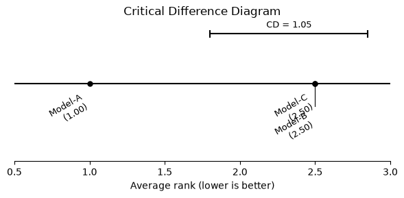
print(f"Friedman p = {freq_result.friedman_p_value:.4f},  CD = {freq_result.cd:.3f}")
freq_result.table[["model_a", "model_b", "rank_diff", "p_value", "significant"]]
Friedman p = 0.0006, CD = 1.048
| model_a | model_b | rank_diff | p_value | significant | |
|---|---|---|---|---|---|
| 0 | Model-A | Model-B | 1.5 | 0.002296 | True |
| 1 | Model-A | Model-C | 1.5 | 0.002296 | True |
| 2 | Model-B | Model-C | 0.0 | 1.000000 | False |
fig = freq_result.plot(title="Critical Difference Diagram")
plt.tight_layout()
plt.show()
Bayesian: posterior probability of superiority#
bayes_result = bench.bayesian_comparison(rope=0.01, random_state=0)
bayes_result.table[["model_a", "model_b", "p_a_better", "p_equiv", "p_b_better"]]
| model_a | model_b | p_a_better | p_equiv | p_b_better | |
|---|---|---|---|---|---|
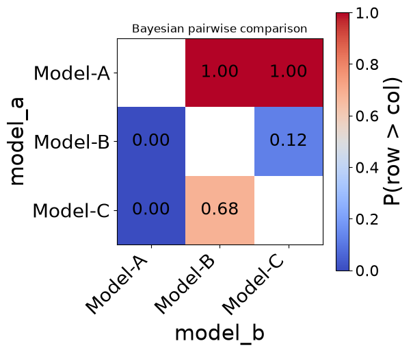
| 0 | Model-A | Model-B | 1.00000 | 0.00000 | 0.0000 |
| 1 | Model-A | Model-C | 1.00000 | 0.00000 | 0.0000 |
| 2 | Model-B | Model-C | 0.12232 | 0.19598 | 0.6817 |
fig = bayes_result.plot(title="Bayesian pairwise comparison")
plt.tight_layout()
plt.show()
Side-by-side: where they agree#
merged = freq_result.table[["model_a", "model_b", "p_value", "significant"]].merge(
    bayes_result.table[["model_a", "model_b", "p_a_better", "p_equiv", "p_b_better"]],
    on=["model_a", "model_b"],
    how="left",
)
merged
| model_a | model_b | p_value | significant | p_a_better | p_equiv | p_b_better | |
|---|---|---|---|---|---|---|---|
| 0 | Model-A | Model-B | 0.002296 | True | 1.00000 | 0.00000 | 0.0000 |
| 1 | Model-A | Model-C | 0.002296 | True | 1.00000 | 0.00000 | 0.0000 |
| 2 | Model-B | Model-C | 1.000000 | False | 0.12232 | 0.19598 | 0.6817 |
For the A–B and A–C pairs, both methods agree: the Nemenyi p-value is below 0.05 and P(A > B) is close to 1. For the B–C pair the two methods diverge slightly:
Frequentist: the rank gap between B and C does not exceed the critical difference, so
significant = False.Bayesian:
p_b_bettermay still be around 0.40, capturing residual uncertainty that a binary significant/not-significant verdict cannot express.
When they diverge#
Divergence typically happens in two situations:
1. Small N (few datasets)#
With only 5–6 datasets, the Nemenyi test rarely rejects. The critical difference is proportional to 1/√N, so as N shrinks the CD grows — at N=5 with three models, the CD covers about 74% of the possible rank range and the bar for significance becomes very high. The Friedman chi-squared approximation also degrades at small N. frequentist_comparison requires at least 5 datasets and raises a ValueError below that. The Bayesian test returns meaningful posteriors at any N because it does not rely on a rank-based approximation.
rows_small = [
    {"model": model, "dataset": d, "metric": "acc", "score": round(float(s), 4)}
    for model, scores in models_scores.items()
    for d, s in zip(datasets[:5], list(scores)[:5])
]
bench_small = evaluma.load_df(
    pd.DataFrame(rows_small),
    model="model", dataset="dataset", metric="metric", score="score",
    norm_ref_low=0.0, norm_ref_high=1.0,
)

freq_small = bench_small.frequentist_comparison(alpha=0.05)
bayes_small = bench_small.bayesian_comparison(rope=0.01, random_state=0)

print("Frequentist (N=5):")
print(freq_small.table[["model_a", "model_b", "p_value", "significant"]].to_string(index=False))
print()
print("Bayesian (N=5):")
print(bayes_small.table[["model_a", "model_b", "p_a_better", "p_equiv", "p_b_better"]].to_string(index=False))
Frequentist (N=5):
model_a model_b  p_value  significant
Model-A Model-B 0.030663         True
Model-A Model-C 0.068887        False
Model-B Model-C 0.946370        False

Bayesian (N=5):
model_a model_b  p_a_better  p_equiv  p_b_better
Model-A Model-B     0.99944  0.00056      0.0000
Model-A Model-C     0.99944  0.00056      0.0000
Model-B Model-C     0.12318  0.17362      0.7032
With N=5 the CD covers most of the rank range, so no pair is likely to clear the significance bar. The Bayesian posteriors still show which model is more likely to win and by how much.
2. Borderline cases near the ROPE#
When two models differ by less than the ROPE (region of practical equivalence), the Bayesian test channels probability into p_equiv. The ROPE defines the score gap below which two models are considered interchangeable — a difference that small is not worth distinguishing regardless of what the test says. The Nemenyi test may still reject the null because it only asks whether the difference is nonzero, not whether it is large enough to matter in practice.
# Models within 0.02 of each other
rng2 = np.random.RandomState(7)
rows_close = [
    {"model": "Close-A", "dataset": d, "metric": "acc", "score": round(float(s), 4)}
    for d, s in zip(datasets, np.clip(rng2.normal(0.70, 0.03, 10), 0, 1))
] + [
    {"model": "Close-B", "dataset": d, "metric": "acc", "score": round(float(s), 4)}
    for d, s in zip(datasets, np.clip(rng2.normal(0.69, 0.03, 10), 0, 1))
]
bench_close = evaluma.load_df(
    pd.DataFrame(rows_close),
    model="model", dataset="dataset", metric="metric", score="score",
    norm_ref_low=0.0, norm_ref_high=1.0,
)

freq_close = bench_close.frequentist_comparison(alpha=0.05)
bayes_close = bench_close.bayesian_comparison(rope=0.05, random_state=0)

print("Frequentist (Nemenyi):")
print(freq_close.table[["model_a", "model_b", "p_value", "significant"]].to_string(index=False))
print()
print("Bayesian (rope=0.05):")
print(bayes_close.table[["model_a", "model_b", "p_a_better", "p_equiv", "p_b_better"]].to_string(index=False))
Frequentist (Nemenyi):
model_a model_b  p_value  significant
Close-A Close-B 0.527089        False

Bayesian (rope=0.05):
model_a model_b  p_a_better  p_equiv  p_b_better
Close-A Close-B     0.01244  0.98756         0.0
Here the Bayesian test may show p_equiv dominating because the models are practically equivalent, while the Nemenyi test might also be insignificant but for a different reason: insufficient power at small N. Note that evaluma uses the same Friedman + Nemenyi path even for k=2, rather than the standalone Wilcoxon special-case from Demšar (2006), so the reported p-value comes from Nemenyi.
Practical guidance#
Use the frequentist path when you need a p-value or CD diagram for a paper or benchmark report; use the Bayesian path when you want a probability statement (“P(A > B) = 0.85”). The frequentist path requires N ≥ 5 datasets, and results at that boundary should be treated cautiously because the Friedman chi-squared approximation is coarse at small N. The Bayesian test returns meaningful posteriors at any N. When two models differ by less than your ROPE, the Bayesian test explicitly captures that practical equivalence; the frequentist test has no way to express it.
Running both in a single workflow#
# Full analysis pipeline
freq_res = bench.frequentist_comparison(alpha=0.05)
bayesian_res = bench.bayesian_comparison(rope=0.01, random_state=0)

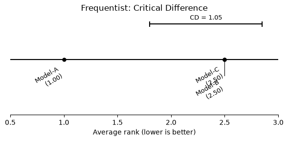
fig = freq_res.plot(title="Frequentist: Critical Difference")
plt.tight_layout()
plt.show()

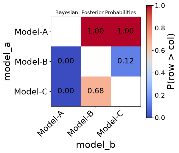
fig = bayesian_res.plot(title="Bayesian: Posterior Probabilities")
plt.tight_layout()
plt.show()
References#
Demšar, J. (2006). Statistical comparisons of classifiers over multiple data sets. JMLR, 7, 1–30.
Holm, S. (1979). A simple sequentially rejective multiple test procedure. Scandinavian Journal of Statistics, 6(2), 65–70.
Benavoli, A., Corani, G., Demšar, J., & Zaffalon, M. (2017). Time for a change: a tutorial for comparing multiple classifiers through Bayesian analysis. JMLR, 18(77), 1–36.