Frequentist Model Comparison: Friedman + Nemenyi / Wilcoxon + Holm

You have run a set of models across a benchmark and sorted the results by IQM score (see IQM Tutorial). Some ranking gaps are wide; others are only a few percentage points. However, before drawing conclusions you want to more carefully assess which observed gaps the data can actually support.

frequentist_comparison() always starts with a Friedman omnibus test to check whether any difference exists, then applies the appropriate post-hoc test:

• All-pairs mode (default): the Demšar (2006) / autorank Friedman + Nemenyi workflow, producing a Critical Difference diagram. Each model is ranked per dataset and the test compares all pairs using those average ranks.

• Reference mode (reference=): pairwise Wilcoxon signed-rank tests against a named baseline with Holm step-down correction. Each model is compared to the baseline using paired normalized score differences directly, not ranks.

Note

This tutorial covers the frequentist approach. For a direct probability statement, “how likely is it that model A outperforms model B on a new task?”, see the Bayesian comparison tutorial. For a comparison of both approaches, see Frequentist vs Bayesian.

import warnings
warnings.filterwarnings("ignore")

import numpy as np
import pandas as pd
import matplotlib.pyplot as plt

import evaluma

1. The Demšar (2006) Protocol

Comparing k > 2 models with pairwise tests directly inflates the false-positive rate. A false positive here means concluding that two models differ significantly when they do not — the more pairs you test, the more likely you are to find one that looks significant by chance alone. The standard correction is a two-step procedure: a Friedman omnibus test first checks whether any classifier differs from the others (a non-parametric equivalent of repeated-measures ANOVA that operates on ranks), and a post-hoc test then identifies which specific pairs differ.

evaluma proceeds to post-hoc testing regardless of the Friedman result, issuing a UserWarning if the Friedman p-value is not below α so you are aware the omnibus test did not support the direction.

Why ranks in the all-pairs branch?

Each dataset \(i\) produces one score per model. Converting to ranks per dataset (rank 1 = highest score) removes scale and direction differences between tasks: a 0.78 accuracy and a 0.78 Jaccard index become comparable once both are replaced by their within-dataset rank.

The average rank of a model across N datasets is the primary summary statistic in the Demšar (2006) all-pairs workflow: a model that consistently ranks first has average rank 1. The reference-mode branch does not use average ranks; it tests paired normalized score differences directly via Wilcoxon signed-rank.

2. Toy Example

A toy benchmark with four models across ten datasets, designed so that some gaps are large and some are not:

rng = np.random.RandomState(34)
datasets = [f"D{i:02d}" for i in range(1, 11)]

scores = {
    "Model-A": np.clip(rng.normal(0.82, 0.03, 10), 0, 1),
    "Model-B": np.clip(rng.normal(0.62, 0.10, 10), 0, 1),
    "Model-C": np.clip(rng.normal(0.47, 0.10, 10), 0, 1),
    "Model-D": np.clip(rng.normal(0.45, 0.10, 10), 0, 1),
}

rows = [
    {"model": m, "dataset": d, "metric": "acc", "score": float(s)}
    for m, sc in scores.items()
    for d, s in zip(datasets, sc)
]
bench = evaluma.load_df(
    pd.DataFrame(rows),
    model="model", dataset="dataset", metric="metric", score="score",
    norm_ref_low=0.0, norm_ref_high=1.0,
)

fig, ax = plt.subplots(figsize=(7, 3.5))
models = list(scores.keys())
means = [scores[m].mean() for m in models]
stds  = [scores[m].std()  for m in models]
x = np.arange(len(models))

ax.bar(x, means, yerr=stds, capsize=4, color="steelblue", alpha=0.6,
       error_kw={"elinewidth": 1.5})
for i, m in enumerate(models):
    ax.scatter(
        np.full(len(scores[m]), i),
        scores[m],
        color="steelblue", s=20, zorder=3, alpha=0.8
    )
ax.set_xticks(x)
ax.set_xticklabels(models)
ax.set_ylabel("Score")
ax.set_ylim(0, 1)
ax.set_title("Per-model scores (mean ± std across 10 datasets)")
plt.tight_layout()
plt.show()

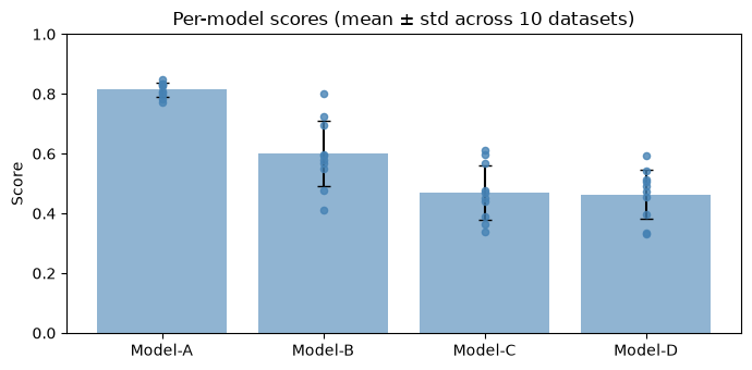
Model-A leads Model-B by roughly 20 points consistently across all datasets. Model-C and Model-D have means only 0.02 apart with high per-dataset variance, with differences reversing direction freely. Model-B holds a ~15-point mean advantage over Model-C and Model-D, though this is borderline given the shared σ ≈ 0.10 noise.

3. All-Pairs Mode: Friedman + Nemenyi

Running the comparison

result = bench.frequentist_comparison(alpha=0.05)
print(f"Friedman  χ² = {result.friedman_statistic:.3f},  p = {result.friedman_p_value:.4f}")
print(f"Critical difference (CD) = {result.cd:.3f}")
result.table

Friedman  χ² = 18.600,  p = 0.0003
Critical difference (CD) = 1.483

	model_a	model_b	rank_diff	p_value	significant
0	Model-A	Model-B	1.3	0.109611	False
1	Model-A	Model-C	2.1	0.001570	True
2	Model-A	Model-D	2.2	0.000799	True
3	Model-B	Model-C	0.8	0.508353	False
4	Model-B	Model-D	0.9	0.402376	False
5	Model-C	Model-D	0.1	0.998155	False

The table has one row per pair. The rank_diff column is \(|\bar{r}_A - \bar{r}_B|\) where \(\bar{r}\) is the average rank across datasets. The p_value comes from the Nemenyi test, which is already FWER-controlled and requires no additional correction.

Column	Meaning
model_a, model_b	The pair being compared
rank_diff	\(|\bar{r}_A - \bar{r}_B|\) — difference in average ranks
p_value	Nemenyi post-hoc p-value (family-wise error rate controlled)
significant	True if p_value < alpha

Note

No p_value_corrected column appears in all-pairs mode. The Nemenyi test uses the Studentized range distribution across all \(k(k-1)/2\) pairs simultaneously, providing FWER control without a secondary correction step. Applying Holm on top would double-correct and be over-conservative.

Critical Difference diagram

The CD diagram (Demšar 2006) converts the result table into a picture of the competitive landscape. The CD scalar marks the minimum rank difference that reaches significance.

fig = result.plot(title="Critical Difference Diagram — toy benchmark, α = 0.05")
plt.tight_layout()
plt.show()

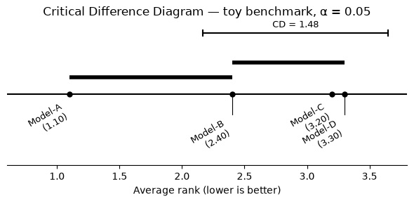
Models are placed on a horizontal axis by average rank (rank 1 = best), so the leftmost model had the highest average rank. A thick horizontal bar connecting two or more models means their rank gap does not exceed the CD scalar; the data cannot confidently separate them. Models with no connecting bar are separated by more than the CD and the Nemenyi p-value is below α. The CD bracket in the top-right corner shows the critical difference on the rank axis: any two models closer than that bracket are not significantly different.

What to look for

Model-A (leftmost) is significantly better than Model-C and Model-D, with rank gaps of 2.1 and 2.2 both exceeding the CD of 1.48. The gap between Model-A and Model-B (rank diff = 1.3) falls just below the CD, so they share a bar and the data cannot confidently separate them. A second bar connects Model-B, Model-C, and Model-D, where no gap reaches significance.

A visible ranking gap is not the same as a statistically supported one. The CD diagram shows which gaps survive the Nemenyi test; the IQM table shows point estimates that do not account for per-dataset variance.

CD scalar formula

The critical difference is:

\[CD = \frac{q_\alpha}{\sqrt{2}} \cdot \sqrt{\frac{k(k+1)}{6N}}\]

where \(q_\alpha\) is the \(\alpha\)-quantile of the Studentized range distribution with \(k\) groups and infinite degrees of freedom, \(k\) is the number of models, and \(N\) is the number of datasets.

from scipy.stats import studentized_range

k = 4   # models
N = 10  # datasets
alpha = 0.05
q_alpha = studentized_range.ppf(1 - alpha, k, df=np.inf) / np.sqrt(2)
cd_manual = q_alpha * np.sqrt(k * (k + 1) / (6 * N))
print(f"CD (manual) = {cd_manual:.4f}")
print(f"CD (result) = {result.cd:.4f}")

CD (manual) = 1.4832
CD (result) = 1.4832

4. Reference Mode: Wilcoxon + Holm

When the question is “which models genuinely improve over a specific baseline?” use reference=. Unlike the all-pairs branch, this mode tests paired normalized score differences directly via Wilcoxon signed-rank, not average ranks. It runs only \(k - 1\) pairwise tests against the reference, then applies Holm step-down correction to control the FWER across those tests.

result_ref = bench.frequentist_comparison(reference="Model-B", alpha=0.05)
print(f"Friedman  χ² = {result_ref.friedman_statistic:.3f},  p = {result_ref.friedman_p_value:.4f}")
result_ref.table

Friedman  χ² = 18.600,  p = 0.0003

	model_a	model_b	w_statistic	p_value	p_value_corrected	significant
0	Model-B	Model-A	1.0	0.003906	0.011719	True
1	Model-B	Model-C	5.0	0.019531	0.039062	True
2	Model-B	Model-D	8.0	0.048828	0.048828	True

Column	Meaning
model_a	The reference model (repeated for every row)
model_b	The model being compared against the reference
w_statistic	Wilcoxon W statistic (sum of the smaller signed-rank group)
p_value	Raw two-sided Wilcoxon p-value
p_value_corrected	Holm step-down corrected p-value — report this
significant	True if p_value_corrected < alpha

fig = result_ref.plot(title="Wilcoxon vs Model-B baseline, α = 0.05")
plt.tight_layout()
plt.show()

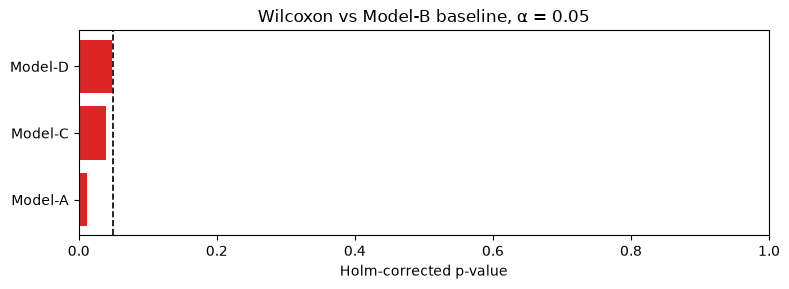
Bars ending to the left of the dashed α line are significantly different from the reference. Grey bars are not.

When to use reference mode vs all-pairs

Scenario	Mode
Understand the full competitive landscape	All-pairs (Nemenyi)
“Which models beat my baseline?”	Reference (Wilcoxon + Holm)

Reference mode uses fewer tests (\(k-1\) vs \(k(k-1)/2\)) and therefore a weaker Holm correction, giving more power for each individual comparison. Models that are borderline in all-pairs mode may reach significance in reference mode.

5. Applying to GeoBench

The IQM ranking tutorial showed ConvNeXt backbones leading by a visible margin. frequentist_comparison tests whether those gaps survive a Friedman + Nemenyi correction across 14 backbones and 19 datasets.

df_raw = pd.read_csv("../../results_and_parameters.csv")

full_coverage = (
    df_raw.groupby("backbone")["dataset"]
    .nunique()
    .pipe(lambda s: s[s == 19].index)
    .tolist()
)
df_geo = df_raw[df_raw["backbone"].isin(full_coverage)].copy()

bench_geo = evaluma.load_df(
    df_geo,
    model="backbone",
    dataset="dataset",
    metric="Metric",
    score="test metric",
    seed="Seed",
    norm_ref_low=0.0,
    norm_ref_high=1.0,
    metric_direction={"biomassters": "min"},
)

result_geo = bench_geo.frequentist_comparison(alpha=0.05)
print(f"Friedman  χ² = {result_geo.friedman_statistic:.3f},  p = {result_geo.friedman_p_value:.4f}")
print(f"CD = {result_geo.cd:.3f}")
fig = result_geo.plot(title="GeoBench — CD diagram, α = 0.05")
plt.tight_layout()
plt.show()

Friedman  χ² = 61.863,  p = 0.0000
CD = 4.552

The CD diagram shows which backbone gaps the data can actually support after the Nemenyi correction. Backbones sharing a bar occupy the same statistical tier, regardless of their IQM ranking position.

Reference mode: testing against a single baseline

result_ref_geo = bench_geo.frequentist_comparison(reference="resnet50", alpha=0.05)
fig = result_ref_geo.plot(title="GeoBench — Wilcoxon vs resnet50, α = 0.05")
plt.tight_layout()
plt.show()

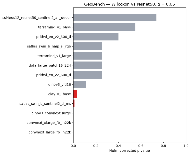
The Holm correction here spans 13 tests (\(k - 1\)) rather than 91 (\(k(k-1)/2\)). Because Holm’s most stringent threshold is \(\alpha / m\) where \(m\) is the number of tests, fewer tests means a less severe correction: in reference mode the hardest hurdle is \(\alpha/13 \approx 0.0038\), compared to \(\alpha/91 \approx 0.00055\) in all-pairs mode, so each individual comparison needs a less extreme p-value to reach significance.

Summary

frequentist_comparison() always runs a Friedman omnibus test first and warns if it is not significant. All-pairs mode uses Nemenyi, which controls FWER across all pairs simultaneously with no secondary correction needed. Reference mode uses Wilcoxon + Holm (fewer tests, a weaker correction, and higher power per comparison) and is the right choice when one specific baseline defines the question. The CD diagram is the standard visualization for all-pairs results: left is better, bars mark indistinguishable groups, and the CD bracket shows the critical difference in rank units. evaluma normalizes scores to [0, 1] per dataset before any statistical test, removing scale and direction differences between metrics.

For a direct comparison of the frequentist and Bayesian approaches, see Frequentist vs Bayesian.

References

• Demšar, J. (2006). Statistical comparisons of classifiers over multiple data sets. Journal of Machine Learning Research, 7, 1–30.

• Holm, S. (1979). A simple sequentially rejective multiple test procedure. Scandinavian Journal of Statistics, 6(2), 65–70.

• Nemenyi, P. (1963). Distribution-free multiple comparisons. PhD thesis, Princeton University.

• Simumba, N. et al. (2026). GEO-Bench: Toward Foundation Models for Earth Monitoring.