Distance from the Best: Improvability Ranking

evaluma offers three complementary ways to rank models, and each answers a different question:

• Aggregate ranking (aggregate_ranking) — what is each model’s typical score level? A point estimate (trimmed mean, mean, or median) of normalized performance.

• ELO ranking (elo_ranking) — how often does each model win head-to-head? A rating derived from pairwise battle frequency across datasets.

• Improvability ranking (improvability_ranking) — how far, in magnitude, is each model from the best? The mean percent error reduction a model would need to match the best model on each dataset.

Improvability is the metric TabArena (Erickson et al., NeurIPS 2025) and BeyondArena (Purucker et al., 2026) both expose as an alternative leaderboard ranking. The two benchmarks are complementary rather than one replacing the other. Unlike a normalized score level, improvability is computed in raw error space: for each dataset, evaluma reconstructs each model’s error, finds the dataset’s best model, and asks what fraction of a model’s current error would have to disappear to tie that best model. That is what “still reducible” means here. The result is bounded in \([0, 100]\%\) and reads directly as “percent of this model’s error that is still left to remove.”

Note

This tutorial contrasts improvability with the aggregate and ELO rankings. For the head-to-head win-rate view in depth, see the ELO ranking tutorial.

import warnings
warnings.filterwarnings("ignore")

import numpy as np
import pandas as pd
import matplotlib.pyplot as plt
import evaluma

1. A benchmark where the three views disagree

The toy benchmark below has four models on six accuracy datasets, split into two thematic halves (D1-D3 and D4-D6).

• Specialist-X is the best method on D1-D3 (0.96) but collapses on D4-D6 (0.55).

• Specialist-Y is the mirror image: best on D4-D6, weak on D1-D3.

• Steady is a strong all-rounder: second on every dataset (0.93 / 0.80).

• Sprinter is a weaker all-rounder: third on every dataset (0.90 / 0.70).

datasets = ["D1", "D2", "D3", "D4", "D5", "D6"]
scores = {
    "Specialist-X": [0.96, 0.96, 0.96, 0.55, 0.55, 0.55],
    "Specialist-Y": [0.55, 0.55, 0.55, 0.96, 0.96, 0.96],
    "Steady":       [0.93, 0.93, 0.93, 0.80, 0.80, 0.80],
    "Sprinter":     [0.90, 0.90, 0.90, 0.70, 0.70, 0.70],
}

rows = [
    {"model": m, "dataset": d, "metric": "acc", "score": float(s)}
    for m, sc in scores.items()
    for d, s in zip(datasets, sc)
]
df = pd.DataFrame(rows)

bench = evaluma.load_df(
    df,
    model="model", dataset="dataset", metric="metric", score="score",
    norm_ref_low=0.0, norm_ref_high=1.0,
)

Scores are already in [0, 1] with explicit bounds, so normalization is the identity. norm_ref_low=0.0, norm_ref_high=1.0 also suppresses the data-driven-bounds warning.

Before looking at any ranking, it helps to see the score pattern directly:

score_matrix = (
    df.pivot(index="model", columns="dataset", values="score")
    .loc[["Specialist-X", "Steady", "Sprinter", "Specialist-Y"], datasets]
)

fig, ax = plt.subplots(figsize=(7, 3.0))
im = ax.imshow(score_matrix.values, cmap="YlOrBr", vmin=0.55, vmax=0.96, aspect="auto")

for i, model in enumerate(score_matrix.index):
    for j, dataset in enumerate(score_matrix.columns):
        value = score_matrix.iloc[i, j]
        color = "white" if value >= 0.88 else "black"
        ax.text(j, i, f"{value:.2f}", ha="center", va="center", color=color)

ax.axvline(2.5, color="white", linewidth=2)
ax.set_xticks(np.arange(len(datasets)))
ax.set_xticklabels(datasets)
ax.set_yticks(np.arange(len(score_matrix.index)))
ax.set_yticklabels(score_matrix.index)
ax.set_title("Two specialists spike on opposite halves; Steady and Sprinter stay consistent")
cbar = fig.colorbar(im, ax=ax, shrink=0.85)
cbar.set_label("Accuracy")
plt.tight_layout()
plt.show()

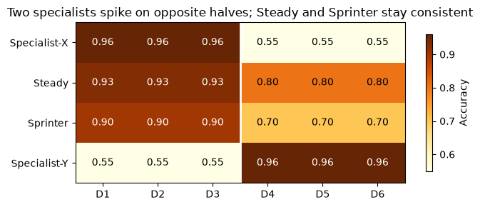
The picture explains why the rankers may disagree: the specialists each have three outright wins and three collapses, while Steady and Sprinter never win but are predictable everywhere.

2. Aggregate ranking: score level

bench.aggregate_ranking(agg="mean").table.round(3)

	model	score
0	Steady	0.865
1	Sprinter	0.800
2	Specialist-Y	0.755
3	Specialist-X	0.755

By mean score, Steady leads (0.865) followed by Sprinter (0.800); the two specialists tie behind them at 0.755 because their three collapse-datasets drag their average down. Consistency wins the aggregate.

3. ELO ranking: head-to-head win frequency

bench.elo_ranking(n_bootstrap=500, random_state=0).table[["model", "ELO"]].round(0)

	model	ELO
0	Steady	1092.0
1	Specialist-X	1000.0
2	Specialist-Y	1000.0
3	Sprinter	908.0

ELO also favors Steady, but it treats the specialists differently from the mean. Because Steady is second on every dataset, it wins most of its pairwise battles and tops the rating (about 1092). The specialists tie at 1000 because each wins exactly half of its pairwise matchups, and Sprinter trails at about 908. ELO measures how often you win, so a specialist’s crushing wins on its home turf count the same as a narrow one.

4. Improvability ranking: distance from the best

Improvability asks a different question: if we freeze this benchmark and try to reduce each model’s error toward the best model on each dataset, what percentage of its current error is still removable? Here the “champion” is simply the model with the smallest error on that dataset.

result = bench.improvability_ranking()
result.table.round(2)

	model	improvability
0	Specialist-X	45.56
1	Specialist-Y	45.56
2	Steady	61.43
3	Sprinter	73.33

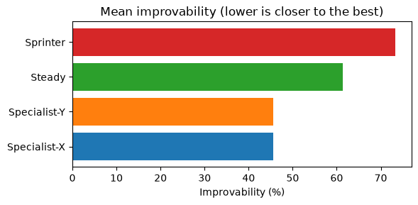
Now the order flips. The two specialists tie for first (45.56%). Steady is third (61.43%) and Sprinter last (73.33%). The reason is direct: on the three datasets where a specialist is already the best model, its improvability is exactly 0, because there is no remaining error to remove relative to that dataset’s best model.

result.plot() renders the ranking as a horizontal bar chart, ascending (best first).

fig = result.plot(figsize=(6, 3), title="Mean improvability (lower is closer to the best)")
plt.tight_layout()
plt.show()

Where the number comes from

Improvability is built in raw error space. For an accuracy dataset the metric’s theoretical optimum is 1.0, so error = 1 - score; the per-dataset best_error is the smallest error achieved by any model on that dataset; and each cell’s improvability is (error - best_error) / error * 100. The .per_dataset table exposes this reconstruction:

result.per_dataset[result.per_dataset["model"].isin(["Specialist-X", "Steady", "Sprinter"])].round(3)

	model	dataset	error	best_error	improvability
0	Specialist-X	D1	0.04	0.04	0.000
1	Specialist-X	D2	0.04	0.04	0.000
2	Specialist-X	D3	0.04	0.04	0.000
3	Specialist-X	D4	0.45	0.04	91.111
4	Specialist-X	D5	0.45	0.04	91.111
5	Specialist-X	D6	0.45	0.04	91.111
12	Sprinter	D1	0.10	0.04	60.000
13	Sprinter	D2	0.10	0.04	60.000
14	Sprinter	D3	0.10	0.04	60.000
15	Sprinter	D4	0.30	0.04	86.667
16	Sprinter	D5	0.30	0.04	86.667
17	Sprinter	D6	0.30	0.04	86.667
18	Steady	D1	0.07	0.04	42.857
19	Steady	D2	0.07	0.04	42.857
20	Steady	D3	0.07	0.04	42.857
21	Steady	D4	0.20	0.04	80.000
22	Steady	D5	0.20	0.04	80.000
23	Steady	D6	0.20	0.04	80.000

For example, Steady scores 0.80 on D4, so its raw error is 0.20. Specialist-Y is the best model there with score 0.96, so the best error is 0.04. Steady’s improvability on D4 is therefore (0.20 - 0.04) / 0.20 = 0.80, or 80%: four-fifths of Steady’s current error on D4 is still removable before it catches the best model on that dataset.

5. Reading the three-way disagreement

To compare the three views fairly, compute ranks from the values themselves rather than from row order. That matters when models are tied.

agg = bench.aggregate_ranking(agg="mean").table.rename(columns={"score": "mean_score"})
agg["agg_rank"] = agg["mean_score"].rank(ascending=False, method="min").astype(int)

elo = bench.elo_ranking(n_bootstrap=500, random_state=0).table[["model", "ELO"]].copy()
elo["elo_rank"] = elo["ELO"].rank(ascending=False, method="min").astype(int)

imp = result.table.copy()
imp["imp_rank"] = imp["improvability"].rank(ascending=True, method="min").astype(int)

summary = (
    agg[["model", "mean_score", "agg_rank"]]
    .merge(elo[["model", "ELO", "elo_rank"]], on="model")
    .merge(imp[["model", "improvability", "imp_rank"]], on="model")
    .sort_values(["agg_rank", "model"])
    .reset_index(drop=True)
)
summary.round({"mean_score": 3, "ELO": 0, "improvability": 2})

	model	mean_score	agg_rank	ELO	elo_rank	improvability	imp_rank
0	Steady	0.865	1	1092.0	1	61.43	3
1	Sprinter	0.800	2	908.0	4	73.33	4
2	Specialist-Y	0.755	3	1000.0	2	45.56	1
3	Specialist-X	0.755	4	1000.0	2	45.56	1

palette = {
    "Specialist-X": "#2563EB",
    "Specialist-Y": "#7C3AED",
    "Steady": "#059669",
    "Sprinter": "#D97706",
}
views = ["Aggregate", "ELO", "Improvability"]
rank_cols = ["agg_rank", "elo_rank", "imp_rank"]

fig, ax = plt.subplots(figsize=(6.2, 3.6))
for _, row in summary.sort_values("model").iterrows():
    y = [row[col] for col in rank_cols]
    ax.plot(views, y, marker="o", linewidth=2.5, markersize=7,
            color=palette[row["model"]], label=row["model"])

ax.set_ylim(4.2, 0.8)
ax.set_ylabel("Rank (1 = best)")
ax.set_title("The specialists climb when the ranking changes from score level to closeness-to-best")
ax.grid(axis="y", alpha=0.25)
ax.legend(loc="center left", bbox_to_anchor=(1.02, 0.5), frameon=False)
plt.tight_layout()
plt.show()

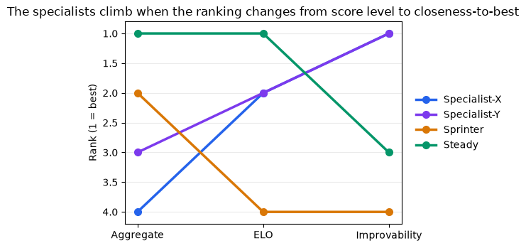
The disagreement is real, but it is not a simple reversal:

• Aggregate and ELO both put Steady first.

• ELO upgrades the specialists from tied third to tied second because each wins three datasets outright.

• Improvability goes further and puts the specialists tied first because it cares about how much error remains relative to the best model on each dataset, not just whether a model wins.

Neither ranking is more correct; they encode different notions of “best.” A model that leads the aggregate but ranks poorly on improvability (like Steady here) is a strong default that is nonetheless never state-of-the-art on any single task. A model that leads improvability but trails the aggregate (like the specialists) may be especially interesting on the datasets where it actually reaches the frontier.

6. Lower-is-better metrics

Improvability is defined in error space, so it handles min metrics directly. For rmse the theoretical optimum is 0.0, so error = score - 0 = score, and the model with the lowest RMSE on each dataset is the best model. The metric direction and optimum are resolved from the built-in registry using each dataset’s metric column.

rmse_rows = [
    {"model": m, "dataset": d, "metric": "rmse", "score": float(s)}
    for m, sc in {
        "Low-error":  [0.10, 0.12, 0.11, 0.09],
        "Mid-error":  [0.20, 0.22, 0.19, 0.21],
        "High-error": [0.40, 0.38, 0.42, 0.41],
    }.items()
    for d, s in zip(["D1", "D2", "D3", "D4"], sc)
]
bench_rmse = evaluma.load_df(
    pd.DataFrame(rmse_rows),
    model="model", dataset="dataset", metric="metric", score="score",
    norm_ref_low=0.0, norm_ref_high=1.0,
)
bench_rmse.improvability_ranking().table.round(2)

	model	improvability
0	Low-error	0.00
1	Mid-error	48.68
2	High-error	73.82

Low-error is the best model on every dataset, so its improvability is 0; the others report how much of their RMSE is still reducible to match it.

For a metric evaluma does not know, the currently supported override is metric_direction={"my_dataset": "min"} when loading. A min override tells improvability the column is already an error bottoming out at 0. Unknown max metrics are not currently supported by improvability_ranking(), because there is no separate user-facing optimum override. A metric that is neither in the registry nor explicitly marked as min raises a clear error only when improvability_ranking() is called, so the benchmark still loads and serves the other methods.

7. Applying It to GeoBench

The synthetic example makes the mechanics obvious. On a real benchmark, the disagreement is usually subtler and more interesting.

GeoBenchV2 evaluates 14 pretrained backbones on 19 geospatial tasks with a mix of Jaccard, F1, accuracy, mAP, and RMSE metrics. This section uses the same results_and_parameters.csv file as the other GeoBench tutorial examples. The question here is not just “who has the highest mean score?” but also “who wins most often?” and “who tends to stay closest to the per-task frontier?”

df_raw = pd.read_csv("../../results_and_parameters.csv")

full_coverage = (
    df_raw.groupby("backbone")["dataset"]
    .nunique()
    .pipe(lambda s: s[s == 19].index)
    .tolist()
)
df_geo = df_raw[df_raw["backbone"].isin(full_coverage)].copy()

bench_geo = evaluma.load_df(
    df_geo,
    model="backbone",
    dataset="dataset",
    metric="Metric",
    score="test metric",
    seed="Seed",
    norm_ref_low=0.0,
    norm_ref_high=1.0,
    metric_direction={"biomassters": "min"},
)

seed="Seed" preserves the per-seed rows for ELO and any other run-level methods, while improvability_ranking() reconstructs raw error from the per-dataset mean scores in the underlying benchmark matrix.

mean_geo = bench_geo.aggregate_ranking(agg="mean").table.rename(columns={"score": "mean"})
mean_geo["mean_rank"] = mean_geo["mean"].rank(ascending=False, method="min").astype(int)

elo_geo = bench_geo.elo_ranking(n_bootstrap=500, random_state=42).table[["model", "ELO"]].copy()
elo_geo["elo_rank"] = elo_geo["ELO"].rank(ascending=False, method="min").astype(int)

imp_geo = bench_geo.improvability_ranking().table.copy()
imp_geo["imp_rank"] = imp_geo["improvability"].rank(ascending=True, method="min").astype(int)

comparison_geo = (
    mean_geo[["model", "mean", "mean_rank"]]
    .merge(elo_geo[["model", "ELO", "elo_rank"]], on="model")
    .merge(imp_geo[["model", "improvability", "imp_rank"]], on="model")
)
comparison_geo["rank_spread"] = (
    comparison_geo[["mean_rank", "elo_rank", "imp_rank"]].max(axis=1)
    - comparison_geo[["mean_rank", "elo_rank", "imp_rank"]].min(axis=1)
)
comparison_geo = comparison_geo[
    ["model", "imp_rank", "improvability", "mean_rank", "elo_rank", "rank_spread"]
]
comparison_geo.sort_values(["imp_rank", "model"]).reset_index(drop=True).round(
    {"improvability": 1}
)

	model	imp_rank	improvability	mean_rank	elo_rank	rank_spread
0	convnext_xlarge_fb_in22k	1	6.0	1	2	1
1	clay_v1_base	2	6.8	3	5	3
2	convnext_large_fb_in22k	3	6.9	2	4	2
3	dinov3_convnext_large	4	7.4	6	1	5
4	terramind_v1_large	5	7.4	5	6	1
5	satlas_swin_b_sentinel2_si_ms	6	7.7	4	7	3
6	dofa_large_patch16_224	7	8.3	8	8	1
7	prithvi_eo_v2_600_tl	8	8.6	9	9	1
8	dinov3_vitl16	9	9.0	7	3	6
9	prithvi_eo_v2_300_tl	10	10.4	10	12	2
10	terramind_v1_base	11	10.8	11	11	0
11	satlas_swin_b_naip_si_rgb	12	11.9	12	10	2
12	ssl4eos12_resnet50_sentinel2_all_decur	13	14.5	13	14	1
13	resnet50	14	16.2	14	13	1

The table is sorted by improvability rank (best first), so the models closest to the task-wise frontier appear at the top.

Three takeaways stand out:

• dinov3_vitl16 disagrees the most: mean rank 7, ELO rank 3, improvability rank 9. It wins enough pairwise matchups to look strong under ELO, but when it loses, it often loses by enough margin that improvability penalizes it.

• dinov3_convnext_large also differs noticeably across views: mean rank 6, ELO rank 1, improvability rank 4. Head-to-head it does extremely well, but its average score level and distance from the best error are less dominant.

• convnext_xlarge_fb_in22k and clay_v1_base look stronger on improvability than on ELO. convnext_xlarge_fb_in22k goes 1 -> 2 -> 1 across mean, ELO, and improvability; clay_v1_base goes 3 -> 5 -> 2. Both stay very close to the task-wise frontier even when they do not top the pairwise win-rate view.

That is exactly why it is useful to report these rankings together. Mean score captures broad score level, ELO captures head-to-head win frequency, and improvability captures closeness to the best error attained on each task.

Summary

• Improvability measures the mean percent error reduction needed to match the per-dataset best model, in raw error space reconstructed from each metric’s direction and theoretical optimum.

• It complements aggregate score level (typical performance) and ELO win frequency (head-to-head dominance). When the three agree, a model’s standing is robust; when they disagree, each is telling you something different about why.

• Lower is better: the per-dataset best model scores 0. A model reaches 0 overall only by being the best on every dataset.

• Known max metrics and known min metrics resolve automatically from the registry. For unknown metrics, the supported fallback is an explicit dataset-level metric_direction="min" override, which treats the raw column as an error metric with optimum 0.

References

• Erickson, N., Purucker, L., Tschalzev, A., Holzmüller, D., Mutalik Desai, P., Salinas, D., & Hutter, F. (2025). TabArena: A Living Benchmark for Machine Learning on Tabular Data. NeurIPS 2025 Datasets and Benchmarks Track (Spotlight). GitHub

• Purucker, L., Tschalzev, A., Erickson, N., Blayer, G., Holzmüller, D., Arazi, A., Pfefferle, A., Tajjar, M., Varoquaux, G., & Hutter, F. (2026). Beyond IID: How General Are Tabular Foundation Models, Really?