Rank Sensitivity: Do Model Rankings Hold Across Conditions?

You have evaluated the same set of models on the same benchmark under two different experimental conditions, such as two optimizers, two data augmentation policies, or two training regimes. Each condition produces an aggregate ranking. A question that now arises, is whether those rankings agree or disagree, and how reliably they due. A single ranking difference between two models could be noise; a systematic reordering could imply that the leaderboard depends on the experimental condition, not on which model is genuinely best.

Note

This tutorial covers rank-correlation analysis between two experimental conditions. For the aggregate rankings that feed into this analysis, see the IQM ranking tutorial. For a direct probability statement (“how likely is Model-A to outperform Model-B on a new task?”), see the Bayesian comparison tutorial.

import warnings
warnings.filterwarnings("ignore")

import numpy as np
import pandas as pd
import matplotlib.pyplot as plt
import evaluma

1. Kendall τ as a ranking agreement statistic

Kendall τ measures agreement between two rankings by counting concordant and discordant pairs. Given two models X and Y, the pair is concordant if both conditions agree on which ranks higher; it is discordant if they disagree. With n models there are C(n, 2) pairs in total.

\[\tau = \frac{C - D}{C + D}\]

where C is the number of concordant pairs and D the number of discordant pairs. τ = 1 means both rankings are identical; τ = −1 means fully reversed; τ = 0 means discordant pairs cancel concordant ones exactly, indicating no agreement beyond chance.

With four models there are C(4, 2) = 6 pairs. If models A and C hold their relative positions across conditions while B and D swap, 3 pairs are concordant (A beats B, A beats C, A beats D) and 3 are discordant (B vs C, B vs D, C vs D each reverse), yielding τ = 0.

Formal definition

For n models ranked under two conditions, let \((x_i, y_i)\) be the rank pair for model \(i\) under conditions A and B respectively. A pair \((i, j)\) is concordant if \((x_i - x_j)\) and \((y_i - y_j)\) have the same sign, discordant if they have opposite signs.

\[\tau = \frac{C - D}{n(n-1)/2}\]

where \(C\) = number of concordant pairs and \(D\) = number of discordant pairs. evaluma passes method="auto" to scipy.stats.kendalltau, which uses the tau-b correction for ties (Kendall, 1945).

evaluma also reports Spearman ρ alongside τ. ρ weights rank gaps by their magnitude rather than counting each pair equally, so it tends to be larger in magnitude than τ when the swap spans multiple rank positions.

2. A 4-model synthetic benchmark

To make the B↔D swap concrete, we construct a benchmark with 4 models, 6 datasets, and two conditions (solver). Model-A ranks first under both optimizers; Model-C ranks third under both. Model-B ranks second under Adam but last under SGD; Model-D ranks last under Adam but second under SGD.

rng = np.random.RandomState(42)
datasets = [f"D{i:02d}" for i in range(1, 7)]

adam_means = {"Model-A": 0.88, "Model-B": 0.74, "Model-C": 0.61, "Model-D": 0.47}
sgd_means  = {"Model-A": 0.87, "Model-B": 0.45, "Model-C": 0.60, "Model-D": 0.73}

rows = []
for solver, means in [("Adam", adam_means), ("SGD", sgd_means)]:
    for model, mu in means.items():
        for d, s in zip(datasets, np.clip(rng.normal(mu, 0.08, 6), 0.0, 1.0)):
            rows.append({"model": model, "dataset": d, "metric": "acc",
                         "score": round(float(s), 4), "solver": solver})
df = pd.DataFrame(rows)

The Adam score matrix shows Model-B comfortably second and Model-D last:

df[df["solver"] == "Adam"].pivot(index="model", columns="dataset", values="score").round(3)

dataset	D01	D02	D03	D04	D05	D06
model
Model-A	0.920	0.869	0.932	1.000	0.861	0.861
Model-B	0.866	0.801	0.702	0.783	0.703	0.703
Model-C	0.629	0.457	0.472	0.565	0.529	0.635
Model-D	0.397	0.357	0.587	0.452	0.475	0.356

The SGD score matrix shows the positions of B and D reversed; Model-A and Model-C remain stable:

df[df["solver"] == "SGD"].pivot(index="model", columns="dataset", values="score").round(3)

dataset	D01	D02	D03	D04	D05	D06
model
Model-A	0.826	0.879	0.778	0.900	0.822	0.847
Model-B	0.402	0.598	0.449	0.365	0.516	0.352
Model-C	0.617	0.443	0.494	0.616	0.659	0.614
Model-D	0.721	0.706	0.612	0.672	0.693	0.815

A grouped bar chart makes the swap visually immediate:

palette = {
    "Model-A": "#2563EB", "Model-B": "#16A34A",
    "Model-C": "#D97706", "Model-D": "#DC2626",
}
model_order = ["Model-A", "Model-B", "Model-C", "Model-D"]

adam_means_obs = df[df["solver"] == "Adam"].groupby("model")["score"].mean()
sgd_means_obs  = df[df["solver"] == "SGD"].groupby("model")["score"].mean()

fig, ax = plt.subplots(figsize=(7, 3.5))
x = np.arange(len(model_order))
width = 0.35

ax.bar(x - width / 2, [adam_means_obs[m] for m in model_order],
       width, label="Adam",
       color=[palette[m] for m in model_order], alpha=0.9)
ax.bar(x + width / 2, [sgd_means_obs[m] for m in model_order],
       width, label="SGD",
       color=[palette[m] for m in model_order], alpha=0.45,
       edgecolor=[palette[m] for m in model_order], linewidth=1.2)

ax.set_xticks(x)
ax.set_xticklabels(model_order)
ax.set_ylabel("Mean accuracy")
ax.set_ylim(0, 1.1)
ax.set_title(
    "Model-B ranks 2nd under Adam, last under SGD; "
    "Model-D is the mirror image"
)
ax.legend(["Adam", "SGD"])
plt.tight_layout()
plt.show()

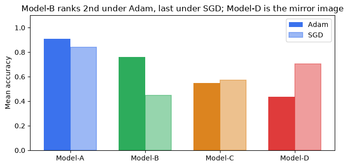
The swap is large: Model-B drops from 0.76 under Adam to 0.45 under SGD, while Model-D rises from 0.44 to 0.70. Model-A and Model-C barely move.

3. Loading with condition_col and running rank sensitivity

load_df accepts a condition_col argument that splits the DataFrame on that column, normalizes each condition independently, and returns a BenchmarkGroup, a dict-keyed container.

bench = evaluma.load_df(
    df,
    model="model", dataset="dataset", metric="metric", score="score",
    norm_ref_low=0.0, norm_ref_high=1.0,
    condition_col="solver",
)
type(bench)

evaluma.benchmark.BenchmarkGroup

bench["Adam"] returns the Benchmark for the Adam condition. Each condition’s scores are normalized relative to that condition’s own reference bounds:

bench["Adam"].scores_.round(3)

	D01	D02	D03	D04	D05	D06
model
Model-A	0.920	0.869	0.932	1.000	0.861	0.861
Model-B	0.866	0.801	0.702	0.783	0.703	0.703
Model-C	0.629	0.457	0.472	0.565	0.529	0.635
Model-D	0.397	0.357	0.587	0.452	0.475	0.356

bench["SGD"] returns the SGD benchmark. Independent normalization matters when conditions have different score ranges or use per-dataset bound dicts. With scalar norm_ref_low=0.0, norm_ref_high=1.0 and scores already in [0, 1], normalization is a pass-through here.

bench.rank_sensitivity("Adam", "SGD") delegates to the two condition benchmarks internally, aligning models and datasets before computing τ:

result = bench.rank_sensitivity("Adam", "SGD", random_state=42)

The result table is sorted by |delta_rank| descending:

result.table

	model	rank_Adam	rank_SGD	delta_rank
0	Model-B	2.0	4.0	2.0
1	Model-D	4.0	2.0	-2.0
2	Model-A	1.0	1.0	0.0
3	Model-C	3.0	3.0	0.0

Model-B and Model-D sit at the top with delta_rank = ±2. Model-A and Model-C have delta_rank = 0: their relative position is unchanged by optimizer choice.

The τ point estimate and its 95% bootstrap CI:

print(f"Kendall τ = {result.tau:.3f}")
print(f"95% bootstrap CI: [{result.tau_ci[0]:.3f}, {result.tau_ci[1]:.3f}]")
print(f"Spearman ρ = {result.rho:.3f}")

Kendall τ = 0.000
95% bootstrap CI: [0.000, 0.333]
Spearman ρ = 0.200

τ = 0.0: the B↔D swap produces exactly 3 concordant and 3 discordant pairs, yielding zero net agreement. The CI [0.00, 0.33] confirms this: no resample produces negative τ, meaning no dataset subsample inverts the B/D swap, but some resamples that happen to draw datasets where B and D perform more similarly produce slight positive agreement. Spearman ρ = 0.20 is larger in magnitude than τ because ρ gives extra weight to the two-position gap between B and D.

Note

If you have two separately built Benchmark objects rather than a single long-format DataFrame, you can call bench_adam.rank_sensitivity(bench_sgd, "Adam", "SGD") directly. The condition_col workflow is the recommended entry point when the data is already in long format.

Before calling rank_sensitivity, you can narrow the comparison with bench.drop_models([...]) or bench.drop_datasets([...]), which return a new BenchmarkGroup with those entries removed from every condition. Subsetting filters cells without re-scaling: the normalization bounds are frozen from the parent, so a retained model’s normalized scores (and its rank relative to the other survivors) do not change when its peers are dropped.

Note

rank_sensitivity ranks models by trimmed_mean by default, matching aggregate_ranking and the IQM/rliable convention, so the two views always agree on the ordering they report. Pass agg="mean" (or agg="median") to opt out — "mean" is the right choice for light-tailed or very-small-N data, where the 25% per-dataset trim discards too much (with 5 datasets only 3 contribute). The chosen mode is recorded on result.agg and appended to the default plot title.

4. The rank scatter plot

.plot() renders rank under Adam on the x-axis against rank under SGD on the y-axis. Each model is a labelled point. The dashed identity line marks perfect agreement. Points above the line rose in rank when moving from Adam to SGD; points below fell.

fig = result.plot(figsize=(5, 5))
plt.tight_layout()
plt.show()

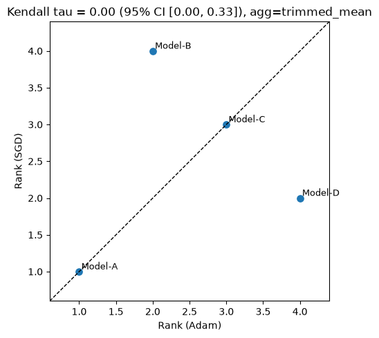
Model-A and Model-C sit on the identity line: their relative positions are unchanged by optimizer choice. Model-B is well below the line: it ranks 2nd under Adam and 4th under SGD. Model-D is the mirror, sitting well above. The distance from the identity line is proportional to |delta_rank|. The plot title reports τ and the 95% CI so that the scatter and the printed values always correspond.

Warning

With fewer than 5 datasets, evaluma raises a UserWarning that the bootstrap CI may be unreliable. Six datasets (as here) are above the threshold but still on the low end; CI width decreases as more datasets are added.

5. What the CI width tells you

The bootstrap CI is constructed by resampling the 6 datasets with replacement 1 000 times, recomputing τ on each resample, and taking the 2.5th–97.5th percentiles. A wide CI does not mean the point estimate is wrong: it means τ is sensitive to which datasets happen to be included. With 6 datasets, many resamples omit one or two entirely while drawing others twice, shifting per-model mean scores enough to occasionally change a rank pair.

To see this, we compare CI width across 4, 6, and 10 datasets drawn from the same score distributions:

for n_datasets in [4, 6, 10]:
    rng_ci = np.random.RandomState(42)
    ds = [f"D{i:02d}" for i in range(1, n_datasets + 1)]
    rows_ci = []
    for solver, means in [("Adam", adam_means), ("SGD", sgd_means)]:
        for model, mu in means.items():
            for d, s in zip(ds, np.clip(rng_ci.normal(mu, 0.08, n_datasets), 0.0, 1.0)):
                rows_ci.append({"model": model, "dataset": d, "metric": "acc",
                                "score": round(float(s), 4), "solver": solver})
    df_ci = pd.DataFrame(rows_ci)
    bench_ci = evaluma.load_df(
        df_ci, model="model", dataset="dataset", metric="metric", score="score",
        norm_ref_low=0.0, norm_ref_high=1.0, condition_col="solver",
    )
    res_ci = bench_ci.rank_sensitivity("Adam", "SGD", random_state=42)
    print(
        f"n={n_datasets:2d}:  τ = {res_ci.tau:.3f},  "
        f"95% CI = [{res_ci.tau_ci[0]:.3f}, {res_ci.tau_ci[1]:.3f}]"
    )

n= 4:  τ = 0.000,  95% CI = [-0.333, 0.333]

n= 6:  τ = 0.000,  95% CI = [0.000, 0.333]

n=10:  τ = 0.000,  95% CI = [0.000, 0.000]

With 4 datasets, the lower bound of the CI turns negative: some resamples omit enough B/D datasets to produce a different ranking pattern, generating occasional negative τ. With 6 datasets, the lower bound reaches zero: the B↔D swap is present in every resample, but a few samples produce slight positive agreement when B and D happen to be drawn from their more similar-performing datasets. With 10 datasets, the CI collapses to [0, 0]: the swap is reproduced so consistently across dataset subsets that τ = 0 on every resample.

τ = 0 with CI [0.00, 0.33] is the actionable finding: the optimizer choice reliably reorders Models B and D, and no dataset subsample contradicts this. A deployment decision that depends on the relative ordering of these two models should not treat Adam and SGD as interchangeable.

Summary

Rankings that appear stable on one benchmark can invert when an experimental condition changes. rank_sensitivity() quantifies this instability using Kendall τ with a 95% bootstrap CI over the dataset axis.

• load_df(condition_col=...) splits a long-format DataFrame by condition, normalizes each independently, and returns a BenchmarkGroup. Call .rank_sensitivity("A", "B") on the group to compare conditions.

• τ = 1 means rankings are identical across conditions; τ = 0 means no net agreement; τ = −1 means fully reversed. Intermediate values reflect partial reordering.

• The CI is computed by resampling datasets with replacement. It measures sensitivity to benchmark composition, not model measurement noise. More datasets narrow the CI.

• Inspect result.table to identify which models drive the instability: large |delta_rank| marks the models whose relative position changes most between conditions.

• When τ is near zero or the CI straddles zero, the leaderboard is condition-dependent. Report separate rankings for each condition, or justify the condition choice on independent grounds before drawing conclusions.

---

For a worked example on real linear-probing benchmark data comparing LBFGS and Adam across geospatial datasets, see [forthcoming].

References

• Kendall, M. G. (1945). The treatment of ties in ranking problems. Biometrika, 33(3), 239–251. https://doi.org/10.1093/biomet/33.3.239

• Agarwal, R., Schwarzer, M., Castro, P. S., Courville, A. C., & Bellemare, M. G. (2021). Deep reinforcement learning at the edge of the statistical precipice. Advances in Neural Information Processing Systems, 34.