Evaluating a Benchmark from a Bayesian Perspective

Suppose you have spent a week running four models across ten datasets. The scores are in, and you now ask youreself which model to choose for a specific task or which to deploy. You compute the means, sort descending, and Model-A wins with 0.73. But Model-B averaged 0.66 — is that gap real? Across ten datasets with natural per-task variation, Model-A might simply have drawn favourable datasets. What you actually want to know is: given a new dataset drawn from the same pool, what is the probability that Model-A outperforms Model-B?

Mean rankings cannot answer that question. Neither, as we will see, can a p-value. This tutorial shows what the Bayesian approach adds, when it matters, and how to use it with evaluma.

Note

This tutorial focuses on the Bayesian perspective. For a full treatment of IQM ranking see IQM tutorial.

import warnings
warnings.filterwarnings("ignore")

import numpy as np
import pandas as pd
import scipy.stats as stats
from itertools import combinations
import tempfile, os

import matplotlib.pyplot as plt
import baycomp

import evaluma

Matplotlib is building the font cache; this may take a moment.

1. The Ranking Fallacy

The natural first move when comparing models is to rank them by mean score. It is fast and readable, but it hides a crucial piece of information.

Consider four models evaluated on ten benchmark datasets.

Mean score hides variance: a model that scores 0.9 on half the datasets and 0.5 on the other half has the same mean as one that scores 0.7 consistently. Ranking by mean cannot tell these apart.

rng = np.random.RandomState(42)
datasets = [f"D{i:02d}" for i in range(1, 11)]
models = ["Model-A", "Model-B", "Model-C", "Model-D"]

scores_raw = {
    "Model-A": np.clip(rng.normal(0.78, 0.09, 10), 0, 1),
    "Model-B": np.clip(rng.normal(0.72, 0.09, 10), 0, 1),
    "Model-C": np.clip(rng.normal(0.68, 0.09, 10), 0, 1),
    "Model-D": np.clip(rng.normal(0.62, 0.09, 10), 0, 1),
}

rows = []
for model, sc in scores_raw.items():
    for d, s in zip(datasets, sc):
        rows.append({"model": model, "dataset": d, "score": round(float(s), 4)})
df_scores = pd.DataFrame(rows)

palette = {
    "Model-A": "#2563EB", "Model-B": "#16A34A",
    "Model-C": "#D97706", "Model-D": "#DC2626",
}

x = np.arange(len(datasets))
width = 0.18
offsets = np.linspace(-1.5, 1.5, 4) * width

fig, ax = plt.subplots(figsize=(9, 4))
for i, model in enumerate(models):
    vals = df_scores[df_scores["model"] == model]["score"].values
    ax.bar(x + offsets[i], vals, width, label=model, color=palette[model])
ax.set_xticks(x)
ax.set_xticklabels(datasets)
ax.set_ylim(0, 1.05)
ax.set_xlabel("Dataset")
ax.set_ylabel("Score")
ax.set_title("Per-dataset scores — four models across ten benchmarks")
ax.legend(title="Model")
plt.tight_layout()
plt.show()

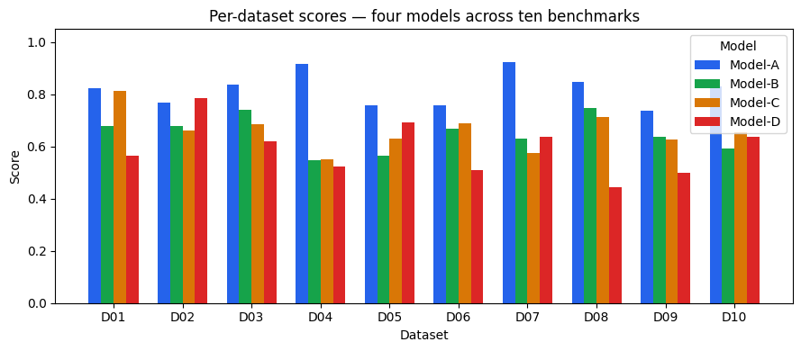
Every model has datasets where it looks strong and others where it drops. Now watch what happens when we collapse this variation to a single number per model:

bench_demo = evaluma.load_df(
    df_scores.assign(metric="acc"),
    model="model", dataset="dataset", metric="metric", score="score",
    norm_ref_low=0.0, norm_ref_high=1.0,
)
bench_demo.aggregate_ranking(agg="mean").table

	model	score
0	Model-A	0.82032
1	Model-C	0.66003
2	Model-B	0.64885
3	Model-D	0.59208

Model-C ranks second and Model-B ranks third — separated by a mean-score gap of 0.011. One percentage point determines which name appears above which in the table. Whether that gap reflects a genuine difference or just sampling noise is exactly what the ranking cannot say.

A ranking answers one question: who scored highest on average. It cannot answer:

• P(Model-A > Model-B) — the probability that A genuinely outperforms B on new data

• How often the difference exceeds a threshold that matters in practice

• Whether two models are interchangeable for this task

Section 2 examines what classical significance tests add, and what they still miss.

2. A Frequentist Approach and What It Can Miss

A p-value asks: if there were no difference between two models, how surprising would this data be? That is a useful sanity check. The Wilcoxon signed-rank test applies this idea to paired benchmark scores: it checks whether the differences across datasets are systematically non-zero, without assuming a particular shape for the distribution.

The signed-rank test ranks the absolute values of the pairwise differences, then checks whether positive and negative differences are balanced. This works without assuming any particular shape for the distribution (non-parametric). Null hypothesis: the median difference is zero.

Below we run all six pairwise Wilcoxon tests and record the p-value alongside the effect size (absolute mean difference).

pair_results = []
for ma, mb in combinations(models, 2):
    sa = df_scores[df_scores["model"] == ma]["score"].values
    sb = df_scores[df_scores["model"] == mb]["score"].values
    diff = sa - sb
    if np.all(np.abs(diff) < 1e-10):
        pval = 1.0
    else:
        _, pval = stats.wilcoxon(diff, zero_method="zsplit")
    pair_results.append({
        "pair": f"{ma} vs {mb}",
        "mean_diff": round(float(np.mean(diff)), 3),
        "abs_effect": round(float(np.abs(np.mean(diff))), 3),
        "p_value": round(float(pval), 4),
        "significant": pval < 0.05,
    })

results_df = pd.DataFrame(pair_results)
results_df

	pair	mean_diff	abs_effect	p_value	significant
0	Model-A vs Model-B	0.171	0.171	0.0020	True
1	Model-A vs Model-C	0.160	0.160	0.0020	True
2	Model-A vs Model-D	0.228	0.228	0.0039	True
3	Model-B vs Model-C	-0.011	0.011	0.6953	False
4	Model-B vs Model-D	0.057	0.057	0.2324	False
5	Model-C vs Model-D	0.068	0.068	0.1934	False

Two results stand out. Model-B vs Model-C is non-significant with a tiny effect — a result consistent with the test’s null, since the mean difference barely exceeds zero. Model-A vs Model-B crosses the significance threshold with an effect of ~0.17, but whether a 17-percentage-point gap matters depends on the application. The test tells you the gap is unlikely to be zero; it says nothing about whether it is large enough to act on.

Important

A p-value answers: “If there were no difference, how surprising would this data be?” For the Wilcoxon signed-rank test, “no difference” means the distribution of paired score differences is symmetric around zero — equivalently, the median difference is zero. That is not the same as: “How probable is it that A genuinely outperforms B?” For a direct probability — the question practitioners actually want answered — you need a Bayesian test.

See also

For a step-by-step guide to frequentist comparison methods including multiple-comparison correction, see the Frequentist tutorial (coming soon).

3. The Bayesian Framework

In Section 2 we computed paired score differences — the per-dataset gap between each pair of models — and asked whether those differences were surprising under a null of zero median difference. The Bayesian approach takes the same paired score differences and asks a different question: what does their distribution tell us about which model is genuinely better? Instead of a binary significant/not-significant verdict, the result is a posterior over three outcomes — A wins, A and B are practically equivalent, B wins — that sum to 1 and directly answer the question you actually want answered.

The method is the Bayesian signed-rank test introduced by Benavoli et al. (2014) and given a comprehensive practitioner treatment in Benavoli et al. (2017). It places a Dirichlet process prior over the distribution of paired score differences — making no assumption about the shape of that distribution beyond exchangeability (the order of datasets does not matter) — and returns a posterior over the three outcomes above. bayesian_comparison() wraps the baycomp implementation of this method. The connection to the signed-rank test from Section 2 is deliberate: both operate on the same paired differences; the Bayesian version replaces the null-hypothesis machinery with a probability statement.

What is the ROPE?

Consider two models that score 85.14% and 85.13% on a dataset. The difference is real but obviously negligible — no practitioner would choose one model over the other on a 0.01-point gap. The Region of Practical Equivalence (ROPE) formalises that judgement: differences smaller than a threshold δ are treated as ties.

δ is called the half-width because the ROPE is the symmetric interval [−δ, +δ]. A difference smaller than δ in either direction is treated as negligible.

On a [0, 1] scale, rope=0.01 means differences smaller than one percentage point are declared ties. The choice encodes domain knowledge: a robotics benchmark might tolerate δ = 0.05, while a medical-imaging benchmark might require δ ≤ 0.01.

Formal definition

For a given ROPE half-width \(\delta\), it returns:

\[p_A = P(\theta_A - \theta_B > \delta), \quad p_{=} = P(|\theta_A - \theta_B| \le \delta), \quad p_B = P(\theta_B - \theta_A > \delta)\]

with \(p_A + p_{=} + p_B = 1\). Here \(\theta_A\) and \(\theta_B\) are the true expected scores for models A and B; \(\delta\) is the ROPE half-width, the threshold below which a score gap is treated as negligible.

Let’s bring this back to the Model-B vs Model-C pair from Section 1, where the ranking separated them by 0.011 points:

# Model-B vs Model-C from the synthetic benchmark above
sb = scores_raw["Model-B"]
sc = scores_raw["Model-C"]
rope_demo = 0.01

p_b_wins, p_eq, p_c_wins = baycomp.two_on_multiple(sb, sc, rope=rope_demo, random_state=42)
print(f"ROPE = {rope_demo}")
print(f"  P(B better)      = {p_b_wins:.3f}")
print(f"  P(equivalent)    = {p_eq:.3f}")
print(f"  P(C better)      = {p_c_wins:.3f}")

ROPE = 0.01
  P(B better)      = 0.384
  P(equivalent)    = 0.018
  P(C better)      = 0.598

The ranking put C ahead of B. The posterior says: we are not confident enough to make that call. Substantial probability lands on equivalence, and neither side dominates.

fig, ax = plt.subplots(figsize=(7, 1.8))
lefts = [0, p_b_wins, p_b_wins + p_eq]
widths_bar = [p_b_wins, p_eq, p_c_wins]
labels = [
    f"P(B better) = {p_b_wins:.3f}",
    f"P(equivalent) = {p_eq:.3f}",
    f"P(C better) = {p_c_wins:.3f}",
]
colors = ["#2563EB", "#9CA3AF", "#DC2626"]
for left, w, label, color in zip(lefts, widths_bar, labels, colors):
    ax.barh(["B vs C"], w, left=left, color=color, label=label)
ax.set_xlim(0, 1)
ax.set_xlabel("Probability")
ax.set_title(f"Bayesian posterior — Model-B vs Model-C (ROPE = {rope_demo})")
ax.legend(loc="upper center", bbox_to_anchor=(0.5, -0.35), ncol=3, fontsize=9)
plt.tight_layout()
plt.show()

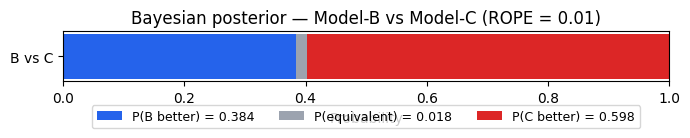
The stacked bar splits the probability budget across three outcomes. With ten datasets and a 0.011-point mean gap, neither side earns a majority — that is the honest answer the data support.

4. Three Patterns in Practice

In practice, Bayesian comparison results fall into three characteristic patterns. Recognising them makes it faster to read a result and decide whether it warrants further scrutiny.

Pattern	Signature	When it occurs
Dominant	\(p_A > 0.95\)	A systematically outperforms B across all datasets
Borderline	\(p_A \approx 0.6,\; p_= \approx 0.3\)	A has a slight edge but outcomes vary per dataset
Tied	\(p_= > 0.95\)	A and B are practically interchangeable

These three patterns are illustrative points on a continuum, not exhaustive categories with hard boundaries — the thresholds (p_A > 0.95 etc.) are rough guides, not precise cutoffs.

Dominant: A wins on nearly every dataset by a margin that exceeds the ROPE. The posterior leaves almost no room for B or equivalence.

Borderline: A has a consistent but small edge. Whether it matters depends on the application — run a sensitivity check with different ROPE values.

Tied: The score differences are so small that the ROPE swallows most of the posterior. Treating these models as interchangeable is well-supported by the data.

We construct three synthetic 15-dataset benchmarks, each designed to exhibit one pattern clearly, then read off what the posteriors reveal.

dsets = [f"ds_{i:02d}" for i in range(1, 16)]

# 1. Dominant: A clearly and consistently ahead of B
rng_dom = np.random.RandomState(42)
a_dom = rng_dom.uniform(0.78, 0.92, 15)
b_dom = rng_dom.uniform(0.15, 0.35, 15)

# 2. Borderline: slight mean difference, high per-dataset variance
rng_bord = np.random.RandomState(7)
a_bord = np.clip(rng_bord.normal(0.65, 0.12, 15), 0, 1)
b_bord = np.clip(rng_bord.normal(0.62, 0.12, 15), 0, 1)

# 3. Tied: A and B produce virtually identical scores
rng_tied = np.random.RandomState(99)
a_tied = rng_tied.uniform(0.65, 0.75, 15)
b_tied = np.clip(a_tied + rng_tied.normal(0, 0.003, 15), 0, 1)


def make_bench_from_arrays(a_scores, b_scores, datasets):
    rows = (
        [{"model": "A", "dataset": d, "metric": "acc", "score": float(s)}
         for d, s in zip(datasets, a_scores)]
        + [{"model": "B", "dataset": d, "metric": "acc", "score": float(s)}
           for d, s in zip(datasets, b_scores)]
    )
    with tempfile.NamedTemporaryFile(suffix=".csv", delete=False, mode="w") as f:
        pd.DataFrame(rows).to_csv(f, index=False)
        path = f.name
    bench = evaluma.load_csv(
        path,
        model="model", dataset="dataset", metric="metric", score="score",
        norm_ref_low=0.0, norm_ref_high=1.0,
    )
    os.unlink(path)
    return bench


bench_dom  = make_bench_from_arrays(a_dom,  b_dom,  dsets)
bench_bord = make_bench_from_arrays(a_bord, b_bord, dsets)
bench_tied = make_bench_from_arrays(a_tied, b_tied, dsets)

r_dom  = bench_dom.bayesian_comparison(rope=0.01, random_state=42)
r_bord = bench_bord.bayesian_comparison(rope=0.05, random_state=42)
r_tied = bench_tied.bayesian_comparison(rope=0.01, random_state=42)

for label, result in [("Dominant", r_dom), ("Borderline", r_bord), ("Tied", r_tied)]:
    row = result.table.iloc[0]
    print(
        f"{label:12s}  "
        f"p_A = {row['p_a_better']:.3f}  "
        f"p_equiv = {row['p_equiv']:.3f}  "
        f"p_B = {row['p_b_better']:.3f}"
    )

Dominant      p_A = 1.000  p_equiv = 0.000  p_B = 0.000
Borderline    p_A = 0.614  p_equiv = 0.319  p_B = 0.067
Tied          p_A = 0.000  p_equiv = 1.000  p_B = 0.000

Already the numbers tell each story: the Dominant case concentrates nearly all probability on A winning; the Tied case concentrates it on equivalence. The Borderline case is the one to scrutinise — A appears to lead, but the probability is spread, not concentrated. The bar charts below show the full probability budget for each pattern side-by-side:

patterns = [
    ("Dominant\n(ROPE=0.01)", r_dom),
    ("Borderline\n(ROPE=0.05)", r_bord),
    ("Tied\n(ROPE=0.01)", r_tied),
]

fig, axes = plt.subplots(1, 3, figsize=(13, 1.6))
colors = ["#2563EB", "#9CA3AF", "#DC2626"]

for ax, (label, result) in zip(axes, patterns):
    row = result.table.iloc[0]
    pa = float(row["p_a_better"])
    pe = float(row["p_equiv"])
    pb = float(row["p_b_better"])
    lefts = [0, pa, pa + pe]
    for left, w, color in zip(lefts, [pa, pe, pb], colors):
        ax.barh([label], [w], left=[left], color=color)
    for left, w, lbl in zip(
        lefts, [pa, pe, pb],
        [f"{pa:.2f}", f"{pe:.2f}", f"{pb:.2f}"]
    ):
        if w > 0.07:
            ax.text(left + w / 2, 0, lbl, ha="center", va="center",
                    fontsize=9, color="white")
    ax.set_xlim(0, 1)
    ax.set_xlabel("Probability")

legend_labels = ["P(A wins)", "P(equivalent)", "P(B wins)"]
handles = [plt.Rectangle((0, 0), 1, 1, color=c) for c in colors]
fig.legend(handles, legend_labels, loc="upper center",
           bbox_to_anchor=(0.5, 0.0), ncol=3, fontsize=9)
plt.tight_layout()
plt.show()

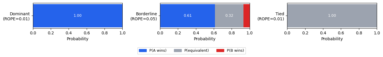
Each bar tells a different story. The Dominant bar is almost entirely blue — the posterior is nearly certain A wins, and rightly so given A scores 0.78–0.92 while B scores 0.15–0.35. The Tied bar is almost entirely grey — the differences are so small the ROPE absorbs them entirely. The Borderline bar is the interesting one: A has a plurality, but probability spreads across all three regions. That spread is not a flaw — it is the honest answer given that A has only a 3-percentage-point mean advantage with substantial per-dataset variance. A mean-score ranking would place A first just as confidently in all three cases; the posterior distinguishes them.

5. Choosing the ROPE

The ROPE is the single most consequential parameter in Bayesian comparison. Set it too small and every comparison looks decisive — even a 0.001-point edge will claim near-certain A-wins. Set it too large and every comparison collapses to equivalence, masking real differences.

As ROPE grows, probability mass migrates from p_A and p_B into p_=: at ROPE = 0, even the smallest consistent edge registers as a decisive win; at ROPE = 0.1, models need a 10-percentage-point gap before the posterior favours either side.

How to choose your ROPE

Step 1 — domain prior. Ask: “Below what score gap would I call these models interchangeable in practice?” Use that as your ROPE. A robotics team deploying monthly might tolerate δ = 0.05; a medical-imaging system reviewed annually might require δ ≤ 0.01.

Step 2 — sensitivity check. Run bayesian_comparison at three ROPE values: your chosen value, half of it, and double it. If p_A swings from > 0.9 to < 0.1 across those three runs, the data do not support a confident claim — report all three results rather than cherry-picking one.

Step 3 — avoid ROPE = 0. With zero ROPE the posterior concentrates all mass on a single outcome as the number of datasets grows, making results brittle even for trivial gaps. Use a small but positive value such as 0.005.

Note

The key sentence: p_A = 0.95 with ROPE = 0.01 means “there is a 95% posterior probability that A beats B by more than one percentage point.” That sentence is precise and directly actionable. A p-value of 0.02 is not.

6. Applying Bayesian Comparison to a Real Benchmark: GeoBench

The sections above built intuition with synthetic data where the ground truth was known. Here we apply the same workflow to a real benchmark where the answer is not obvious in advance.

GeoBench evaluates pretrained visual feature extractors — called backbones — on 19 geospatial remote sensing tasks spanning land cover classification, crop detection, and scene understanding. A backbone is a network such as ResNet-50 or a Vision Transformer, pretrained on large datasets and then fine-tuned for each downstream task. The benchmark covers 14 such backbones. Because task metrics differ in scale and direction (some tasks use Jaccard Index, one uses RMSE), raw scores cannot be compared directly — which is exactly why normalisation matters here.

Driving question: Which backbones genuinely outperform resnet50, and which merely appear ahead in the mean-score ranking?

6a. Loading the data

import pandas as pd
import evaluma

df_raw = pd.read_csv("../../results_and_parameters.csv")

# Keep only the 14 backbones with full dataset coverage (all 19 datasets)
full_coverage = (
    df_raw.groupby("backbone")["dataset"]
    .nunique()
    .pipe(lambda s: s[s == 19].index)
    .tolist()
)
df = df_raw[df_raw["backbone"].isin(full_coverage)].copy()

bench = evaluma.load_df(
    df,
    model="backbone",
    dataset="dataset",
    metric="Metric",
    score="test metric",
    seed="Seed",
    norm_ref_low=0.0,
    norm_ref_high=1.0,
    metric_direction={"biomassters": "min"},
)

evaluma averages across seeds automatically when a seed column is provided, giving one score per (model, dataset) pair.

biomassters uses RMSE (lower is better). Setting metric_direction={"biomassters": "min"} negates that column before normalisation so all scores point in the same direction.

6b. All-pairs comparison

Use this to survey the full competitive landscape — which backbone is genuinely best, and which pairs are statistically indistinguishable?

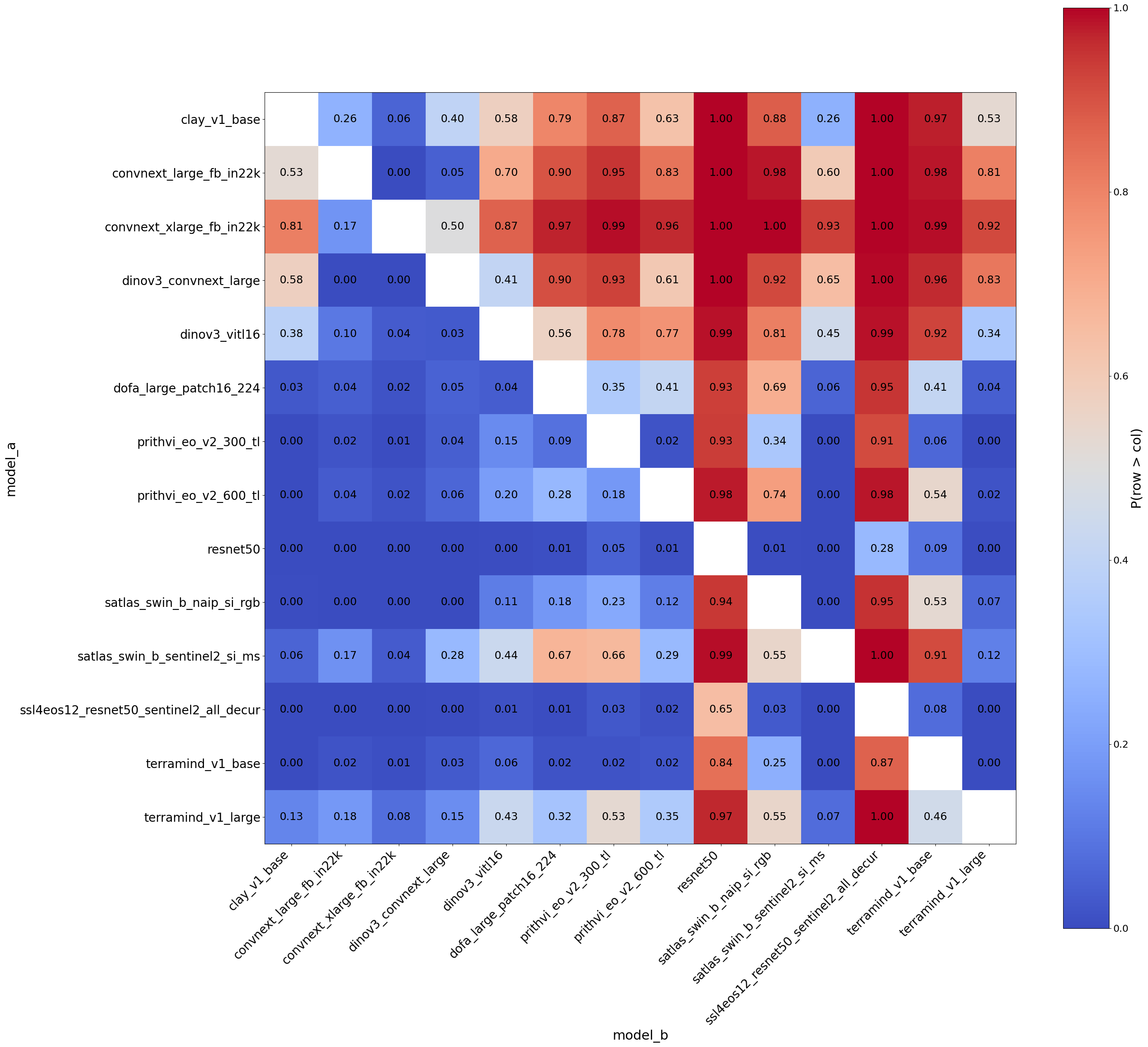
result_all = bench.bayesian_comparison(rope=0.01, random_state=42)
result_all.plot()
plt.tight_layout()
plt.show()

6c. Focused comparison against a baseline

As an alternative mode, you can explicitly compute probabilities against a chosen baseline. The result will be a bar chart that directly answers: which backbones genuinely outperforms the baseline (resnet50 in this case), which are equivalent, and which fall behind?

result = bench.bayesian_comparison(rope=0.01, reference="resnet50", random_state=42)
result.table

	model_a	model_b	p_a_better	p_equiv	p_b_better
0	resnet50	clay_v1_base	0.00044	0.00020	0.99936
1	resnet50	convnext_large_fb_in22k	0.00000	0.00000	1.00000
2	resnet50	convnext_xlarge_fb_in22k	0.00000	0.00000	1.00000
3	resnet50	dinov3_convnext_large	0.00000	0.00004	0.99996
4	resnet50	dinov3_vitl16	0.00498	0.00968	0.98534
5	resnet50	dofa_large_patch16_224	0.00816	0.05864	0.93320
6	resnet50	prithvi_eo_v2_300_tl	0.05114	0.01454	0.93432
7	resnet50	prithvi_eo_v2_600_tl	0.01332	0.00732	0.97936
8	resnet50	satlas_swin_b_naip_si_rgb	0.00520	0.05258	0.94222
9	resnet50	satlas_swin_b_sentinel2_si_ms	0.00000	0.01112	0.98888
10	resnet50	ssl4eos12_resnet50_sentinel2_all_decur	0.28390	0.07026	0.64584
11	resnet50	terramind_v1_base	0.09362	0.06322	0.84316
12	resnet50	terramind_v1_large	0.00494	0.02922	0.96584

result.plot()
plt.tight_layout()
plt.show()

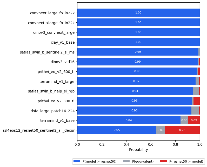
6d. Reading the results

Most backbones earn decisive wins — they consistently outperform resnet50 by more than one normalised percentage point across 19 diverse tasks, and the posterior leaves almost no room for doubt.

Two backbones land in a borderline zone, and they differ in character. terramind_v1_base leans clearly ahead of resnet50, but with enough per-dataset variation that the posterior stops short of certainty. ssl4eos12_resnet50_sentinel2_all_decur is more genuinely ambiguous: it looks ahead in the mean-score ranking, but per-dataset outcomes vary enough that the posterior spreads substantially across both sides.

No backbone sits near practical equivalence — the differences from resnet50 are consistent enough that the ROPE absorbs very little probability mass across the board.

This is the information a mean ranking cannot surface. A backbone ranked near the top by mean score might still belong to the borderline zone if its per-dataset outcomes are inconsistent; one ranked lower might earn a decisive win if its advantage is small but reliable. Only the per-dataset distribution of differences, not the aggregate mean, determines which.

The normalisation step is what makes the ROPE threshold uniform across tasks. evaluma normalises each dataset independently to [0, 1] before comparison, so ROPE = 0.01 means the same thing on a Jaccard Index task and on the RMSE task. Without that step, a raw-score ROPE would need separate tuning for every metric.

Per-dataset min-max normalisation means the Bayesian test operates on a common [0, 1] scale regardless of the original metric. A ROPE of 0.01 therefore means the same thing on every dataset.

Summary

• Mean rankings tell you who scored highest on average; they cannot tell you whether the gap is real or how confident you should be in the ordering.

• The Wilcoxon test tells you whether a difference is statistically unlikely to be zero, but not how probable it is that one model genuinely outperforms another.

• Bayesian comparison returns three probabilities — A wins, equivalent, B wins — that sum to 1 and directly answer the question practitioners actually ask.

• The ROPE encodes the score gap below which two models are considered interchangeable. Always run a sensitivity check across at least three ROPE values before reporting a result.

• The three patterns — Dominant, Borderline, Tied — give a fast interpretation framework for a continuum of results. Borderline results deserve the most scrutiny and benefit most from a sensitivity check.

References

• Benavoli, A., Corani, G., Mangili, F., Zaffalon, M., & Ruggeri, F. (2014). A Bayesian Wilcoxon signed-rank test based on the Dirichlet process. In E. P. Xing & T. Jebara (Eds.), Proceedings of the 31st International Conference on Machine Learning (ICML 2014), PMLR 32(2), 1026–1034. https://proceedings.mlr.press/v32/benavoli14.html

• Benavoli, A., Corani, G., Demšar, J., & Zaffalon, M. (2017). Time for a change: a tutorial for comparing multiple classifiers through Bayesian analysis. Journal of Machine Learning Research, 18(77), 1–36. https://jmlr.org/papers/v18/16-305.html

• baycomp documentation