Ranking Models by Head-to-Head Dominance: ELO from TabArena#
A model can lead an aggregate ranking while losing most of its direct pairwise comparisons. This happens when a small number of exceptional datasets pull its mean score above competitors that perform more consistently across the rest of the benchmark. Aggregate statistics summarize trimmed performance across all tasks; ELO-style ranking asks a different question: which model wins most often when placed head-to-head against each opponent on each dataset? The method is adapted from TabArena (Erickson et al., NeurIPS 2025), where it was introduced as a complement to aggregate ranking on tabular benchmarks.
Note
This tutorial covers ELO ranking from pairwise battle outcomes. For IQM with bootstrap confidence intervals, including the GeoBench data loading pattern reused here, see the IQM ranking tutorial. For probabilistic pairwise statements (how likely is Model-A to outperform Model-B on a new dataset?) see the Bayesian comparison tutorial.
import warnings
warnings.filterwarnings("ignore")

import numpy as np
import pandas as pd
import matplotlib.pyplot as plt
import evaluma
1. Battles: the atomic unit#
A battle is a single pairwise comparison between two models on one dataset: one model wins (outcome 1), the other loses (outcome 0), or they draw (outcome 0.5). With \(M\) models and \(N\) datasets there are \(\binom{M}{2} \times N\) battles in total. Equal-dataset weighting is enforced by assigning each dataset a total weight of 1 distributed across all model pairs that contested it, so a dataset with many competing models does not dominate the ELO fit.
To illustrate the gap between aggregate ranking and head-to-head dominance, the toy benchmark below places one model at ≈ 0.97 on two datasets while scoring below all others on the remaining five.
rng = np.random.RandomState(42)
datasets = [f"D{i:02d}" for i in range(1, 8)]

scores_dict = {
    "Model-A": np.concatenate([rng.uniform(0.96, 0.98, 2), rng.uniform(0.49, 0.51, 5)]),
    "Model-B": np.concatenate([rng.uniform(0.07, 0.09, 2), rng.uniform(0.71, 0.73, 5)]),
    "Model-C": np.concatenate([rng.uniform(0.05, 0.07, 2), rng.uniform(0.61, 0.63, 5)]),
    "Model-D": np.concatenate([rng.uniform(0.03, 0.05, 2), rng.uniform(0.51, 0.53, 5)]),
}

rows = [
    {"model": m, "dataset": d, "metric": "acc", "score": float(s)}
    for m, sc in scores_dict.items()
    for d, s in zip(datasets, sc)
]
df_toy = pd.DataFrame(rows)

bench = evaluma.load_df(
    df_toy,
    model="model", dataset="dataset", metric="metric", score="score",
    norm_ref_low=0.0, norm_ref_high=1.0,
)
bench.scores_.round(3)
| D01 | D02 | D03 | D04 | D05 | D06 | D07 | |
|---|---|---|---|---|---|---|---|
| model | |||||||
| Model-A | 0.967 | 0.979 | 0.505 | 0.502 | 0.493 | 0.493 | 0.491 |
| Model-B | 0.087 | 0.082 | 0.724 | 0.710 | 0.729 | 0.727 | 0.714 |
| Model-C | 0.054 | 0.054 | 0.616 | 0.620 | 0.619 | 0.616 | 0.622 |
| Model-D | 0.033 | 0.036 | 0.517 | 0.519 | 0.526 | 0.514 | 0.520 |
Model-A scores ≈ 0.97 on D01 and D02 but ≈ 0.50 on D03–D07, where Models B, C, and D all score higher. Model-B is weak on D01–D02 (≈ 0.08) but leads D03–D07 at ≈ 0.72.
Mean aggregation ranks Model-A first because adding two near-perfect scores to five middling ones produces a higher average than adding two very low scores to five strong ones.
mean_result = bench.aggregate_ranking(agg="mean")
mean_result.table.round(3)
| model | score | |
|---|---|---|
| 0 | Model-A | 0.633 |
| 1 | Model-B | 0.539 |
| 2 | Model-C | 0.457 |
| 3 | Model-D | 0.381 |
Model-A’s mean score (0.633) leads the field. Model-B, which beats Model-A on five of seven datasets, sits second at 0.539. The aggregate flattens a structure that the win-rate matrix makes visible.
2. Win-rate matrix#
bench.elo_ranking() computes ELO ratings and simultaneously builds the win-rate matrix from all pairwise battles.
result = bench.elo_ranking(n_bootstrap=1000, random_state=42)
result.plot_winrate() renders the M×M fraction-of-datasets-won for every model pair.
fig = result.plot_winrate(
    figsize=(5, 4),
    title="Win-rate matrix: fraction of datasets where row model beats column model",
)
plt.tight_layout()
plt.show()
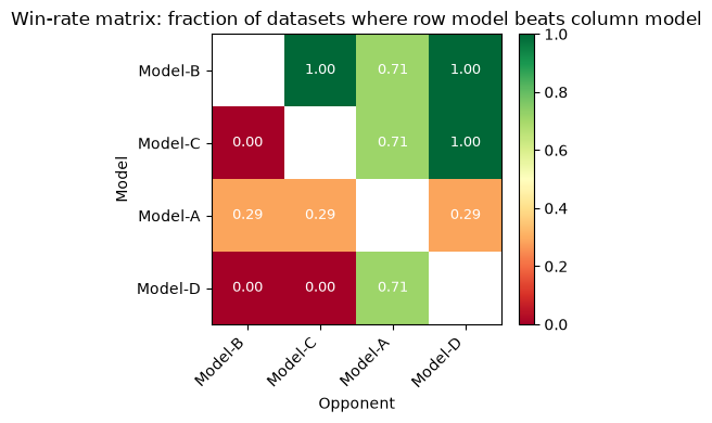
Model-A’s row is 0.29 across every column: it wins only on D01 and D02 (2 out of 7 datasets = 0.29) regardless of which other model it faces. Model-B’s row is the opposite: 0.71 against Model-A (winning on D03–D07) and 1.00 against Model-C and Model-D, which it beats on all seven datasets.
The matrix also surfaces a counterintuitive result. Model-D, which ranks last by mean score (0.381), beats Model-A on five of seven datasets (D03–D07, where D ≈ 0.52 and A ≈ 0.50). A model that leads by aggregate can lose to last-place competitors when its high mean is driven by a small number of datasets where it dominates and everyone else collapses.
3. MLE ELO ratings with bootstrap CIs#
ELO ratings are fit by maximum likelihood, following TabArena. The ELO model sets the probability that model \(i\) beats model \(j\) to \(1 / \left(1 + \text{base}^{-(R_i - R_j)/\text{scale}}\right)\), where \(R\) is the vector of ratings and the constants \(\text{base}=10\), \(\text{scale}=400\) fix the convention that a 400-point gap corresponds to 10:1 odds. This is a logistic regression: each battle contributes one row with \(+\ln(\text{base})\) in model \(i\)’s column and \(-\ln(\text{base})\) in model \(j\)’s column, weighted to enforce equal dataset contributions. Folding \(\ln(\text{base})\) into the design matrix (rather than using \(\pm 1\) entries) makes the fitted coefficients land directly on the ELO scale, so the final ratings are simply \(\text{scale} \times \text{coefficients}\). Ties are expanded into two half-weight rows, one with outcome 1 and one with outcome 0, so that a draw contributes half a win and half a loss to each side.
Bootstrap confidence intervals resample battles within each dataset. For each of the 1000 replicates, the set of battles that belong to dataset \(k\) is resampled with replacement; ELO is then refit on the reassembled battles table. This captures uncertainty about which datasets drive the ranking: if a few datasets dominate a model’s ELO, the CI will be wide.
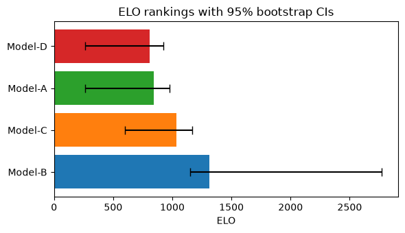
result.plot() renders the ratings as a horizontal bar chart with 95% CI error bars.
fig = result.plot(
    figsize=(6, 3.5),
    title="ELO rankings with 95% bootstrap CIs",
)
plt.tight_layout()
plt.show()
result.table lists the point estimates and 95% CI bounds in descending ELO order.
result.table.round(1)
| model | ELO | CI_low | CI_high | |
|---|---|---|---|---|
| 0 | Model-B | 1312.0 | 1151.4 | 2771.3 |
| 1 | Model-C | 1037.4 | 601.1 | 1170.2 |
| 2 | Model-A | 842.3 | 265.7 | 977.4 |
| 3 | Model-D | 808.3 | 260.2 | 922.9 |
Model-B leads at ELO 1312, well above Model-C (1037) and Model-A (842), which sits close to Model-D (808) despite having the highest mean score. Model-B’s CI is wide: bootstrap replicates that draw mainly from D01–D02 (where B scores only ≈ 0.08) produce very low resampled ratings, while replicates that draw mainly from D03–D07 produce very high ones. Model-C and Model-A have overlapping CIs, so the data do not confidently separate their ELO positions.
4. tie_threshold: treating near-ties as draws#
By default, any non-zero score difference produces a decisive battle. A normalized difference of 0.02 is treated the same as one of 0.50, even though the first is likely within measurement noise. tie_threshold sets a minimum gap: pairs whose normalized scores differ by at most the threshold produce a draw rather than a win or loss.
bench.elo_ranking(tie_threshold=0.05) converts 10 of the 42 battles to draws (the A vs D pairs on D03–D07 and several C–D pairs where scores differ by less than 0.05 on the [0, 1] normalized scale).
result_t = bench.elo_ranking(tie_threshold=0.05, random_state=42)
result_t.table.round(1)
| model | ELO | CI_low | CI_high | |
|---|---|---|---|---|
| 0 | Model-B | 1224.3 | 1114.0 | 1389.6 |
| 1 | Model-C | 1043.2 | 944.3 | 1146.1 |
| 2 | Model-A | 938.9 | 823.7 | 1031.3 |
| 3 | Model-D | 793.5 | 677.2 | 863.6 |
The ELO spread narrows: Model-B drops from 1312 to 1224 as some of its dominant wins are softened to partial credit, and the other models follow a similar pattern. The ranking is unchanged.
Note
tie_threshold operates on the [0, 1] normalized score scale. A value of 0.05 means “within 5 percentage points on the normalized benchmark scale.” This is analogous to the rope parameter in bench.bayesian_comparison(), which also treats normalized-score differences below a threshold as practically equivalent.
5. calibration_model: anchoring the scale#
Raw ELO ratings carry no inherent absolute meaning: the scale depends on the initialization constant and the specific battles. calibration_model shifts all ratings so that a designated anchor lands at exactly 1000, making results interpretable relative to a known baseline and comparable across benchmark runs.
result_c = bench.elo_ranking(calibration_model="Model-B", random_state=42)
result_c.table.round(1)
| model | ELO | CI_low | CI_high | |
|---|---|---|---|---|
| 0 | Model-B | 1000.0 | 1000.0 | 1000.0 |
| 1 | Model-C | 725.5 | -1092.7 | 952.9 |
| 2 | Model-A | 530.3 | -1469.0 | 779.1 |
| 3 | Model-D | 496.3 | -1438.7 | 733.2 |
With Model-B anchored to 1000, Model-C sits at 726 and Model-A at 530. The calibration anchor’s CI collapses to [1000, 1000] by construction; the CIs for other models widen because they now carry all the fitting uncertainty relative to that fixed point.
6. Multi-seed battles with raw_runs#
When the benchmark is loaded with a seed column, elo_ranking() generates one set of battles per (dataset, seed) combination rather than one per dataset. Each dataset still contributes total weight 1 regardless of how many seeds are available, so a dataset with three seeds does not dominate one with one seed. Bootstrap resampling draws within (dataset, seed) groups, which typically narrows CIs when per-seed variance is low.
The multi-seed benchmark below extends the same 4-model, 7-dataset structure with 3 seeds per cell and model-specific per-seed variance.
rng2 = np.random.RandomState(99)
outlier_datasets = {"D01", "D02"}
model_sigma = {
    "Model-A": {"outlier": 0.02, "stable": 0.04},
    "Model-B": {"outlier": 0.01, "stable": 0.02},
    "Model-C": {"outlier": 0.01, "stable": 0.01},
    "Model-D": {"outlier": 0.01, "stable": 0.03},
}

rows_seeded = []
for m, sc in scores_dict.items():
    sigs = model_sigma[m]
    for d, base in zip(datasets, sc):
        sigma = sigs["outlier"] if d in outlier_datasets else sigs["stable"]
        for seed_id in [1, 2, 3]:
            score = float(np.clip(base + rng2.normal(0, sigma), 0.0, 1.0))
            rows_seeded.append(
                {"model": m, "dataset": d, "metric": "acc", "score": score, "seed": seed_id}
            )
df_seeded = pd.DataFrame(rows_seeded)

bench_runs = evaluma.load_df(
    df_seeded,
    model="model", dataset="dataset", metric="metric", score="score",
    seed="seed",
    norm_ref_low=0.0, norm_ref_high=1.0,
)
bench_runs.elo_ranking() automatically uses the per-seed battles path because bench_runs carries raw runs.
result_runs = bench_runs.elo_ranking(random_state=42)
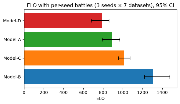
fig = result_runs.plot(
figsize=(6, 3.5),
title="ELO with per-seed battles (3 seeds × 7 datasets), 95% CI",
)
plt.tight_layout()
plt.show()
result_runs.table shows how the CI bounds compare to the single-seed run.
result_runs.table.round(1)
| model | ELO | CI_low | CI_high | |
|---|---|---|---|---|
| 0 | Model-B | 1308.4 | 1217.3 | 1475.3 |
| 1 | Model-C | 1015.5 | 954.3 | 1073.0 |
| 2 | Model-A | 888.4 | 790.5 | 968.6 |
| 3 | Model-D | 787.8 | 681.3 | 860.6 |
Compared to the single-seed run, all CIs are narrower. With 3 seeds per dataset, each dataset contributes 3 groups of battles to the bootstrap rather than 1; resampling within 21 groups (3 seeds × 7 datasets) rather than 7 constrains the estimate more tightly. The ranking is unchanged: Model-B leads and Model-A ranks third despite its high mean score.
7. Applying to GeoBenchV2#
GeoBenchV2 (Simumba et al., 2026) evaluates 14 pretrained backbone models on 19 geospatial datasets. The data loading is identical to the IQM tutorial; elo_ranking() automatically uses the per-seed battles path because bench_geo is loaded with seed="Seed".
df_raw = pd.read_csv("../../results_and_parameters.csv")

full_coverage = (
    df_raw.groupby("backbone")["dataset"]
    .nunique()
    .pipe(lambda s: s[s == 19].index)
    .tolist()
)
df_geo = df_raw[df_raw["backbone"].isin(full_coverage)].copy()

bench_geo = evaluma.load_df(
    df_geo,
    model="backbone",
    dataset="dataset",
    metric="Metric",
    score="test metric",
    seed="Seed",
    norm_ref_low=0.0,
    norm_ref_high=1.0,
    metric_direction={"biomassters": "min"},
)
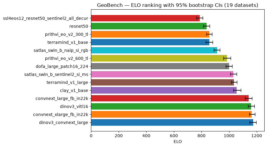
bench_geo.elo_ranking() fits MLE ELO from per-seed battles across 19 datasets and 14 backbones. The example uses 200 bootstrap replicates to keep docs execution time bounded; for a final analysis, increase n_bootstrap if you need tighter CI estimates.
elo_geo = bench_geo.elo_ranking(n_bootstrap=200, random_state=42)

fig = elo_geo.plot(
    figsize=(9, 5),
    title="GeoBench — ELO ranking with 95% bootstrap CIs (19 datasets)",
)
plt.tight_layout()
plt.show()
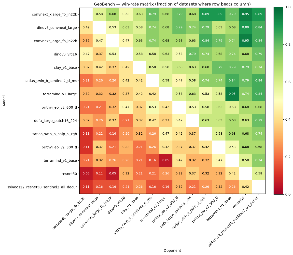
elo_geo.plot_winrate() renders the 14×14 pairwise win-rate heatmap.
fig = elo_geo.plot_winrate(
    figsize=(12, 11),
    title="GeoBench — win-rate matrix (fraction of datasets where row beats column)",
)
plt.tight_layout()
plt.show()
IQM rank vs ELO rank#
Placing IQM and ELO rankings side by side identifies backbones whose aggregate score and head-to-head consistency tell different stories.
iqm_geo = bench_geo.iqm_ranking(random_state=42)

elo_ranks = elo_geo.table[["model", "ELO"]].copy()
elo_ranks.insert(0, "elo_rank", range(1, len(elo_ranks) + 1))

iqm_ranks = iqm_geo.table[["model", "IQM"]].copy()
iqm_ranks.insert(0, "iqm_rank", range(1, len(iqm_ranks) + 1))

comparison = elo_ranks.merge(iqm_ranks, on="model")
comparison["rank_diff"] = comparison["elo_rank"] - comparison["iqm_rank"]
comparison["ELO"] = comparison["ELO"].round(1)
comparison["IQM"] = comparison["IQM"].round(3)
comparison.sort_values("elo_rank").reset_index(drop=True)
| elo_rank | model | ELO | iqm_rank | IQM | rank_diff | |
|---|---|---|---|---|---|---|
| 0 | 1 | dinov3_convnext_large | 1174.1 | 3 | 0.542 | -2 |
| 1 | 2 | convnext_xlarge_fb_in22k | 1163.5 | 1 | 0.544 | 1 |
| 2 | 3 | dinov3_vitl16 | 1158.6 | 4 | 0.538 | -1 |
| 3 | 4 | convnext_large_fb_in22k | 1143.0 | 2 | 0.543 | 2 |
| 4 | 5 | clay_v1_base | 1056.1 | 5 | 0.533 | 0 |
| 5 | 6 | terramind_v1_large | 1036.2 | 6 | 0.531 | 0 |
| 6 | 7 | satlas_swin_b_sentinel2_si_ms | 1030.7 | 7 | 0.530 | 0 |
| 7 | 8 | dofa_large_patch16_224 | 1000.9 | 8 | 0.527 | 0 |
| 8 | 9 | prithvi_eo_v2_600_tl | 985.8 | 9 | 0.518 | 0 |
| 9 | 10 | satlas_swin_b_naip_si_rgb | 913.0 | 10 | 0.518 | 0 |
| 10 | 11 | terramind_v1_base | 857.1 | 11 | 0.511 | 0 |
| 11 | 12 | prithvi_eo_v2_300_tl | 856.6 | 12 | 0.508 | 0 |
| 12 | 13 | resnet50 | 837.1 | 14 | 0.473 | -1 |
| 13 | 14 | ssl4eos12_resnet50_sentinel2_all_decur | 787.1 | 13 | 0.477 | 1 |
The bottom ten positions are stable across both methods. The top four are reshuffled. By IQM, convnext_xlarge_fb_in22k leads narrowly (0.544) over convnext_large_fb_in22k (0.543), with dinov3_convnext_large third (0.542). By ELO, dinov3_convnext_large leads and convnext_large_fb_in22k drops to fourth.
The IQM differences at the top are under 0.002, so the ELO reversal reflects genuine head-to-head consistency rather than rounding noise in a tight aggregate race. convnext_large_fb_in22k ranks second by IQM but wins fewer head-to-head battles than dinov3_convnext_large and dinov3_vitl16. The win-rate matrix identifies which specific dataset comparisons drive this split.
When ELO and IQM agree on a backbone’s position, that position is robust to both the choice of aggregation method and the distribution of head-to-head outcomes. When they disagree, the win-rate matrix is the right tool to investigate whether the disagreement is driven by a few specialized datasets or a broader pattern across the benchmark.
Summary#
ELO ranking and IQM aggregate capture different aspects of benchmark performance: IQM measures trimmed mean score while ELO measures head-to-head dominance. When they agree the ranking is robust; when they disagree, the win-rate matrix identifies which datasets drive the split.
Read the win-rate matrix before reading ELO ratings. A model with a high average win-rate is consistently competitive; a uniform low win-rate row signals that the model’s aggregate score is driven by a few exceptional datasets rather than broad performance.
tie_thresholdprevents trivially small score differences from producing decisive battle outcomes. Set it to a value consistent with your metric’s measurement precision, on the [0, 1] normalized scale.calibration_modelfixes the absolute scale so ratings are interpretable relative to a known baseline, useful when comparing across benchmark runs or communicating to a wider audience.When
raw_runsare available (multiple seeds per dataset),elo_ranking()automatically generates per-seed battles and resamples within (dataset, seed) groups, which typically narrows CIs compared to single-seed bootstrapping.For a probabilistic pairwise statement (“how likely is Model-X to outperform Model-Y on a new task?”) use
bench.bayesian_comparison()as shown in the Bayesian comparison tutorial.
References#
Erickson, N., Purucker, L., Tschalzev, A., Holzmüller, D., Mutalik Desai, P., Salinas, D., & Hutter, F. (2025). TabArena: A Living Benchmark for Machine Learning on Tabular Data. NeurIPS 2025 Datasets and Benchmarks Track (Spotlight). GitHub
Agarwal, R., Schwarzer, M., Castro, P. S., Courville, A. C., & Bellemare, M. G. (2021). Deep reinforcement learning at the edge of the statistical precipice. Advances in Neural Information Processing Systems, 34.
Simumba, N. et al. (2026). GEO-Bench: Toward Foundation Models for Earth Monitoring.